3. Linear classification, Optimization, SGD

Part of CS231n Winter 2016

---

Lecture 3: Loss Functions and Optimization

Andrej keeps pushing the data-driven pipeline forward: once we commit to learning from examples, we need loss functions that quantify failure and optimization routines that search weight space efficiently.

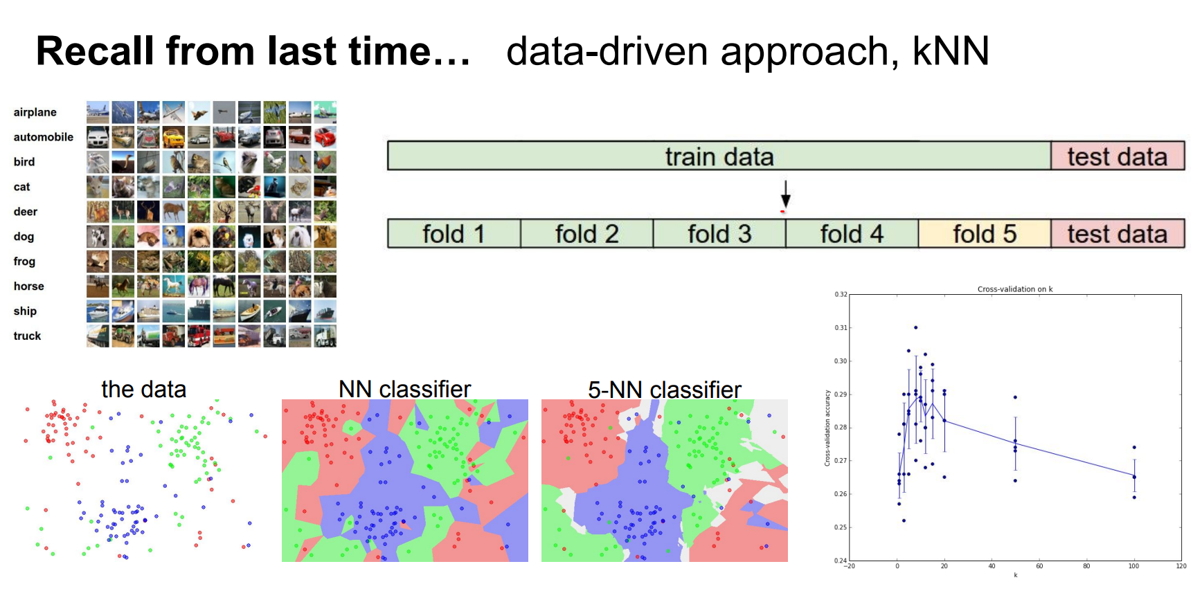
Recap: Data-Driven Classification

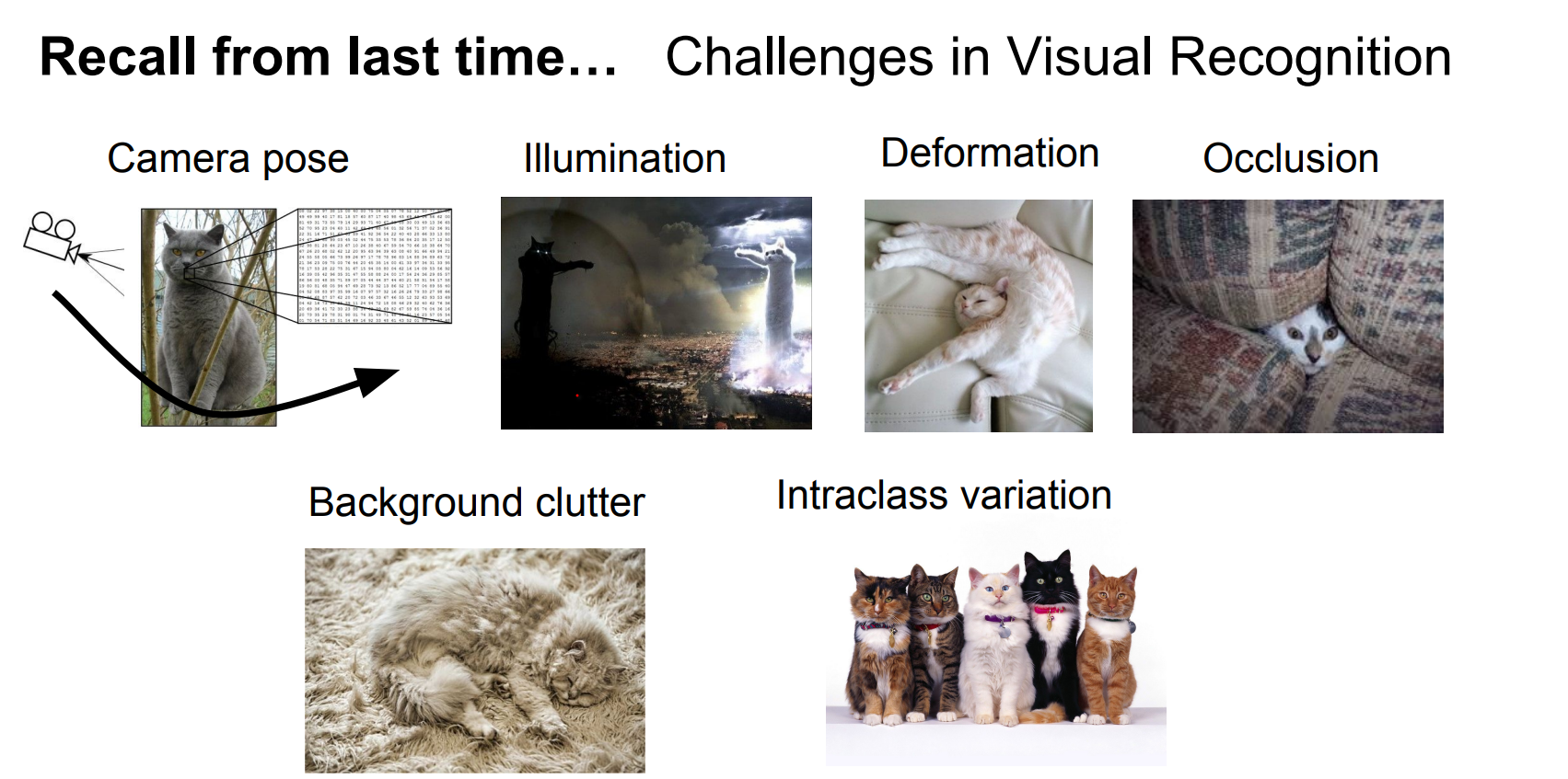
• We build image classifiers such as CIFAR-10 by matching high-dimensional templates or, more intuitively, by finding separating hyperplanes in feature space.

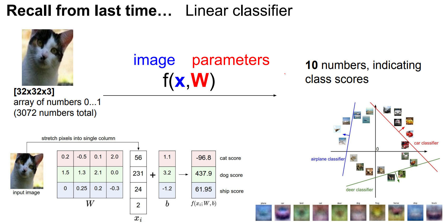
We are trying to find a function.

• The workflow stays the same: define a loss over the training set, then minimize it with respect to the weights using some optimizer.

We can interpret the situation as, matching templates or images being in high dimensional space and classifiers separating them.

In other words, we are trying to find weights that are good for all of our classes.

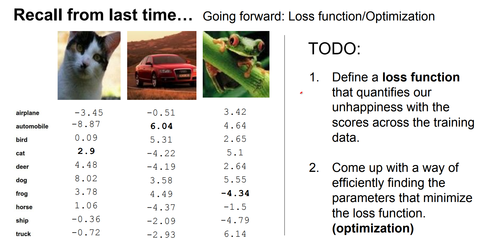
1. Define a loss function that quantifies our unhappiness with the scores across the training data.
2. Come up with a way of efficiently finding the parameters that minimize the loss function. (optimization)

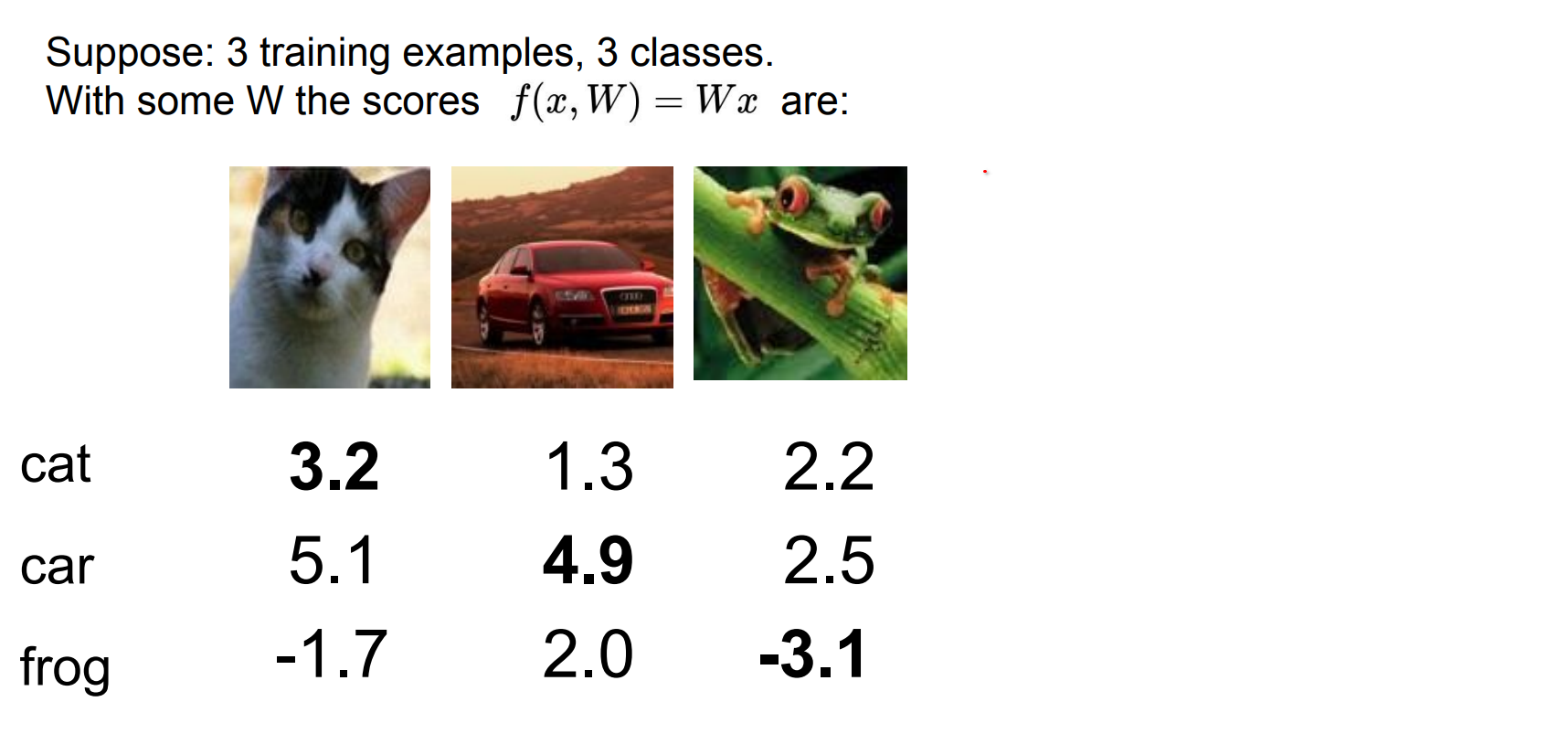
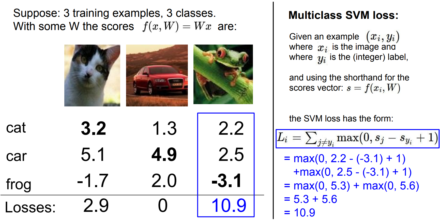
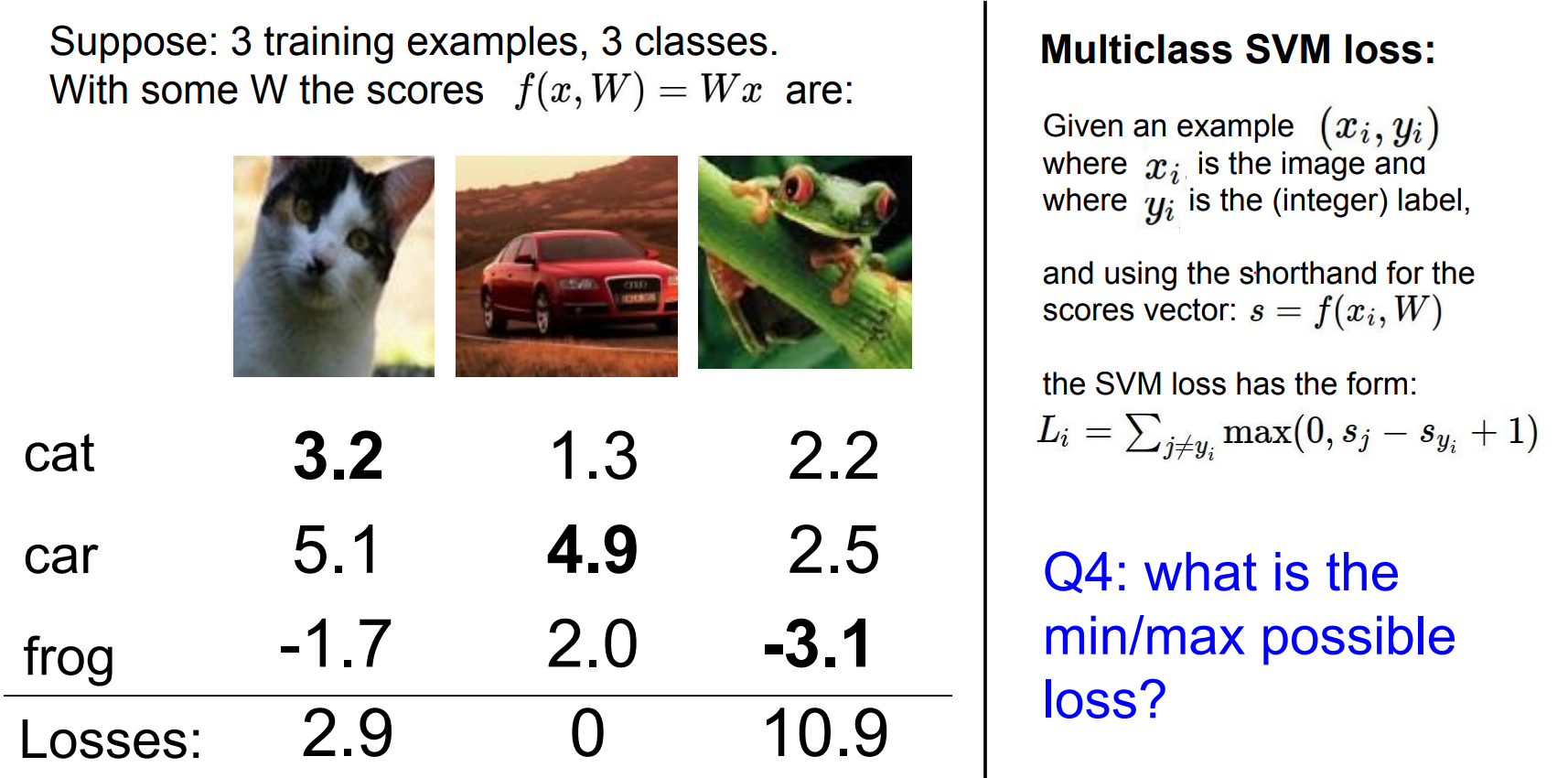
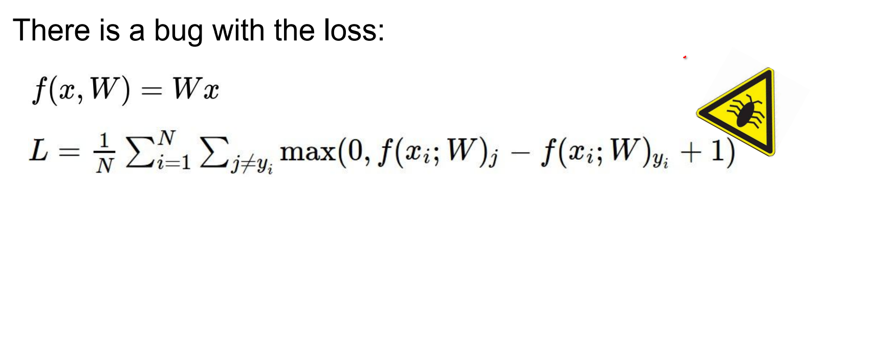
Multi-class SVM Loss

Intuition

• Compare the score of the correct class against every incorrect class.
• Introduce a safety margin (usually 1); violations incur positive loss, otherwise clamp to 0.
• Sum the margin violations across all off-target classes.

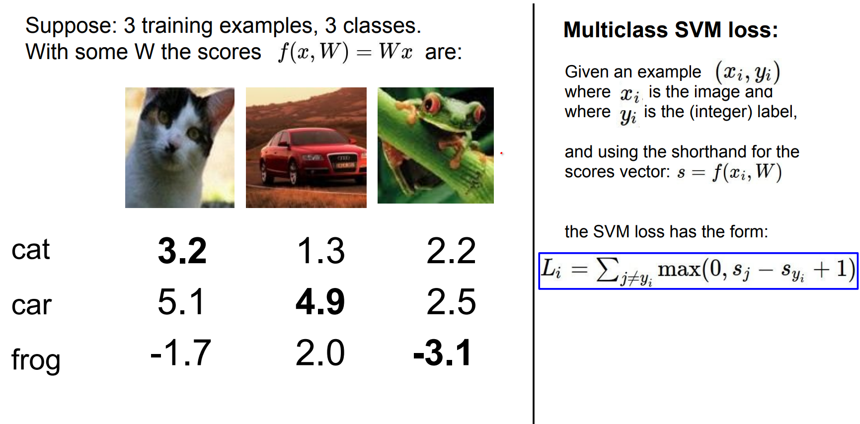
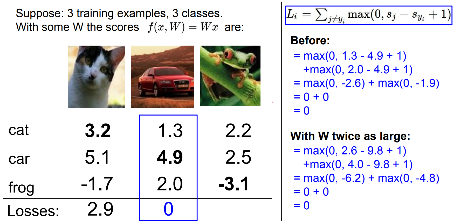
Let:

• \(s_j\) be the score of a wrong class (car, frog, ...) (class score where the class is not the Ground Truth).
• \(s_{y_i}\) be the score of the ground-truth class.

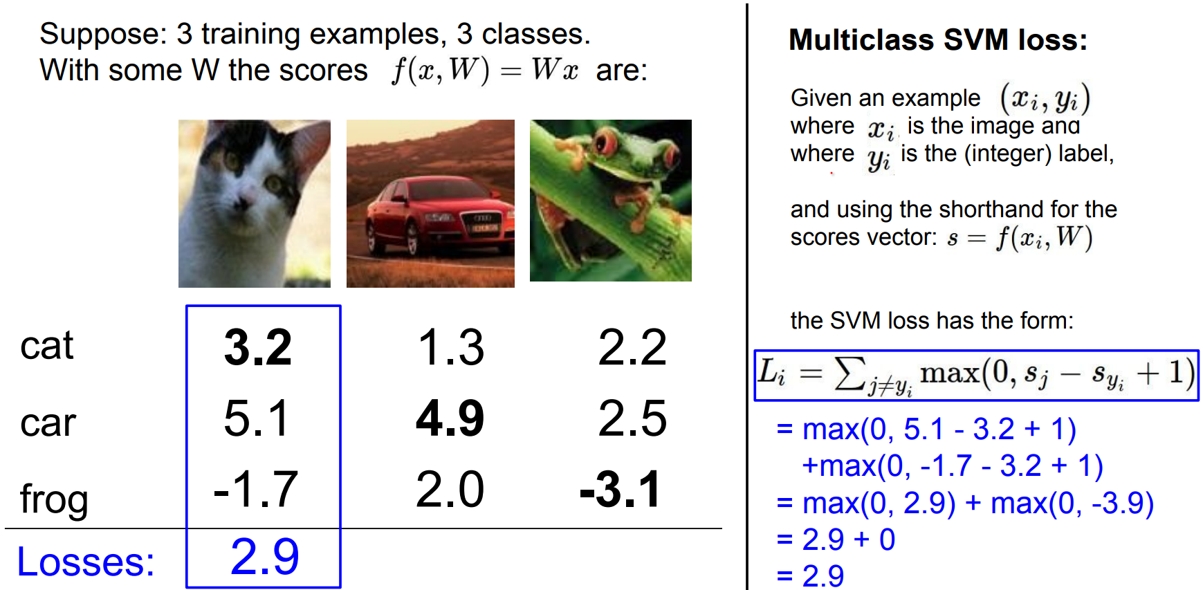
Example interpretation:

• For the first image, all incorrect classes should be <= 2.2 if the correct class is 3.2.

• The car class at 5.1 contributes 2.9 to the loss, while frog contributes 0.

• Total loss: 2.9

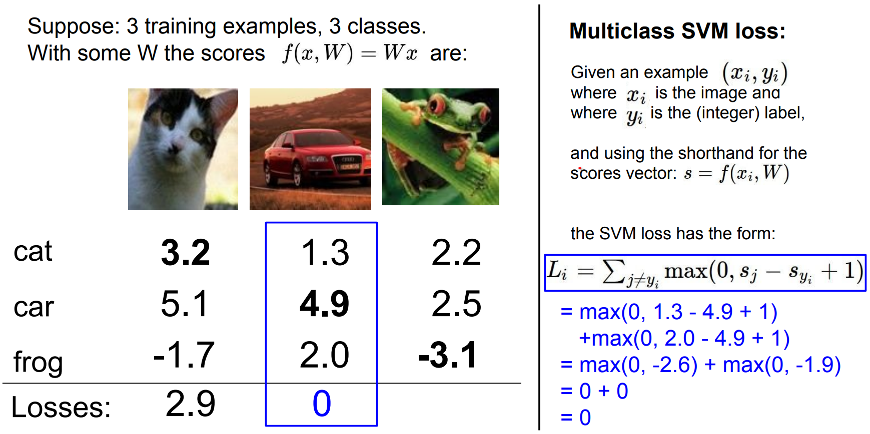
Loss of 0, because the car score is higher than other classes by at least 1.0

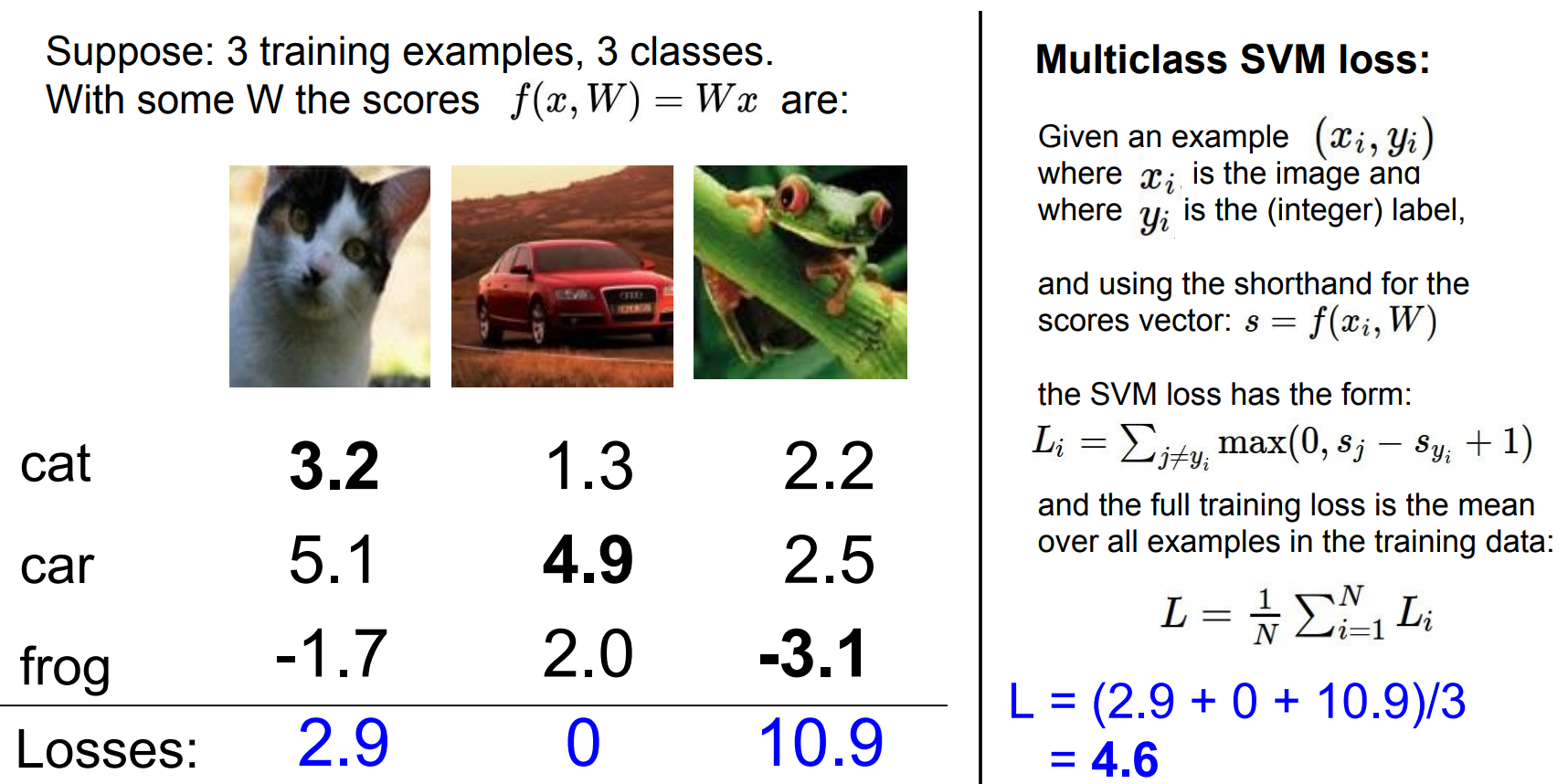
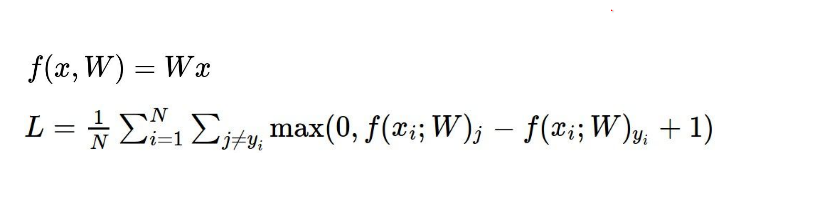
Combined Objective

• What happens if we sum over all classes, including \(j = y_i\) ?
  You simply add 1 to the loss because \(max(0, s_y - s_y + 1) = 1\). The optimum shifts by a constant but gradients stay the same.

max(0 , s_j - s_yi + 1) 
# would become
max(0, 1)
# which would be
1

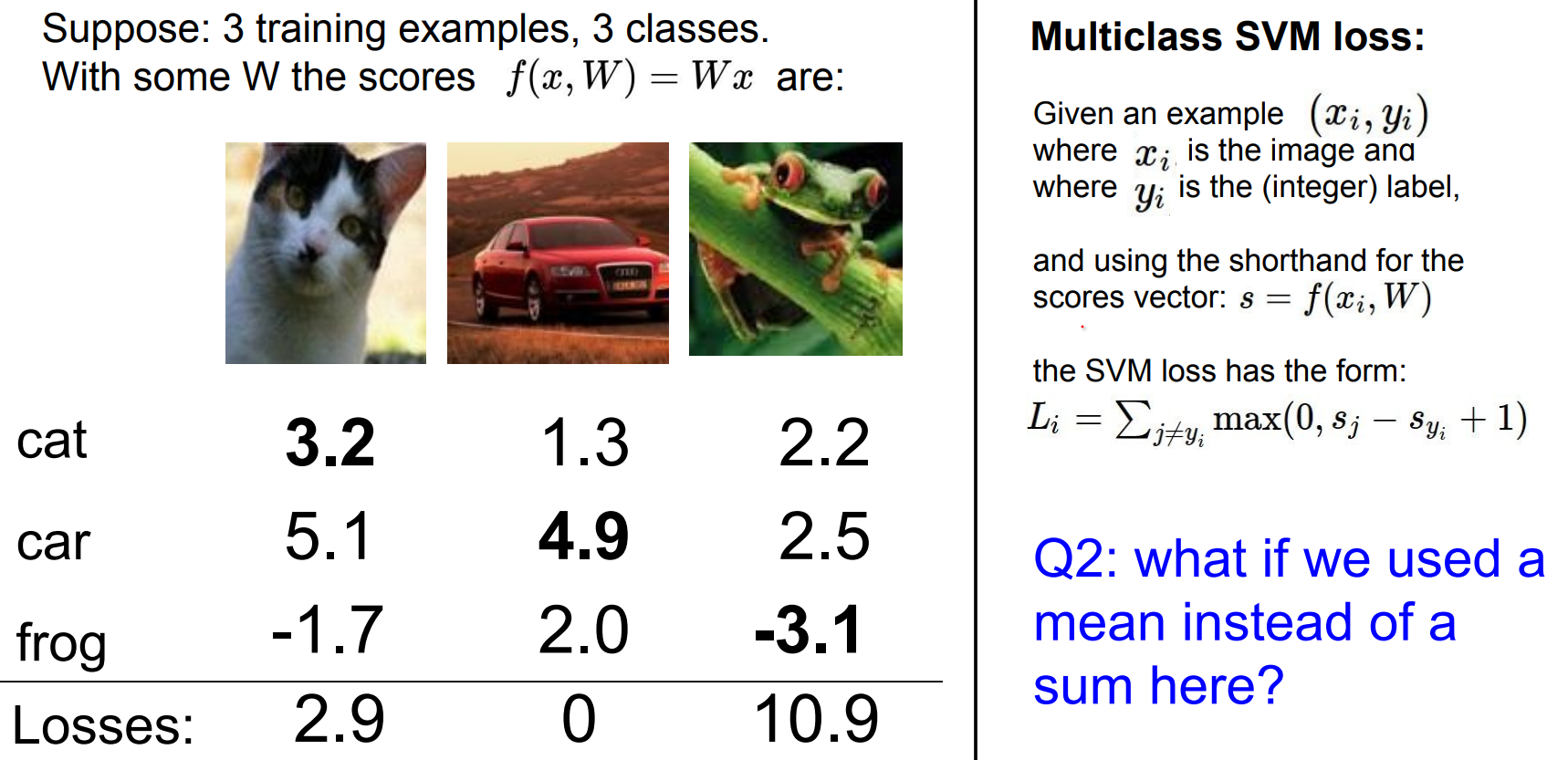
• What if we average instead of summing?
  If we used mean, the loss would be lower (3 classes 1/3 added). In the end we are going to minimize the W over that loss, your solution does not change.

So the scale changes (e.g., divide by the number of classes), but when we later minimize over W the optimum is unchanged.

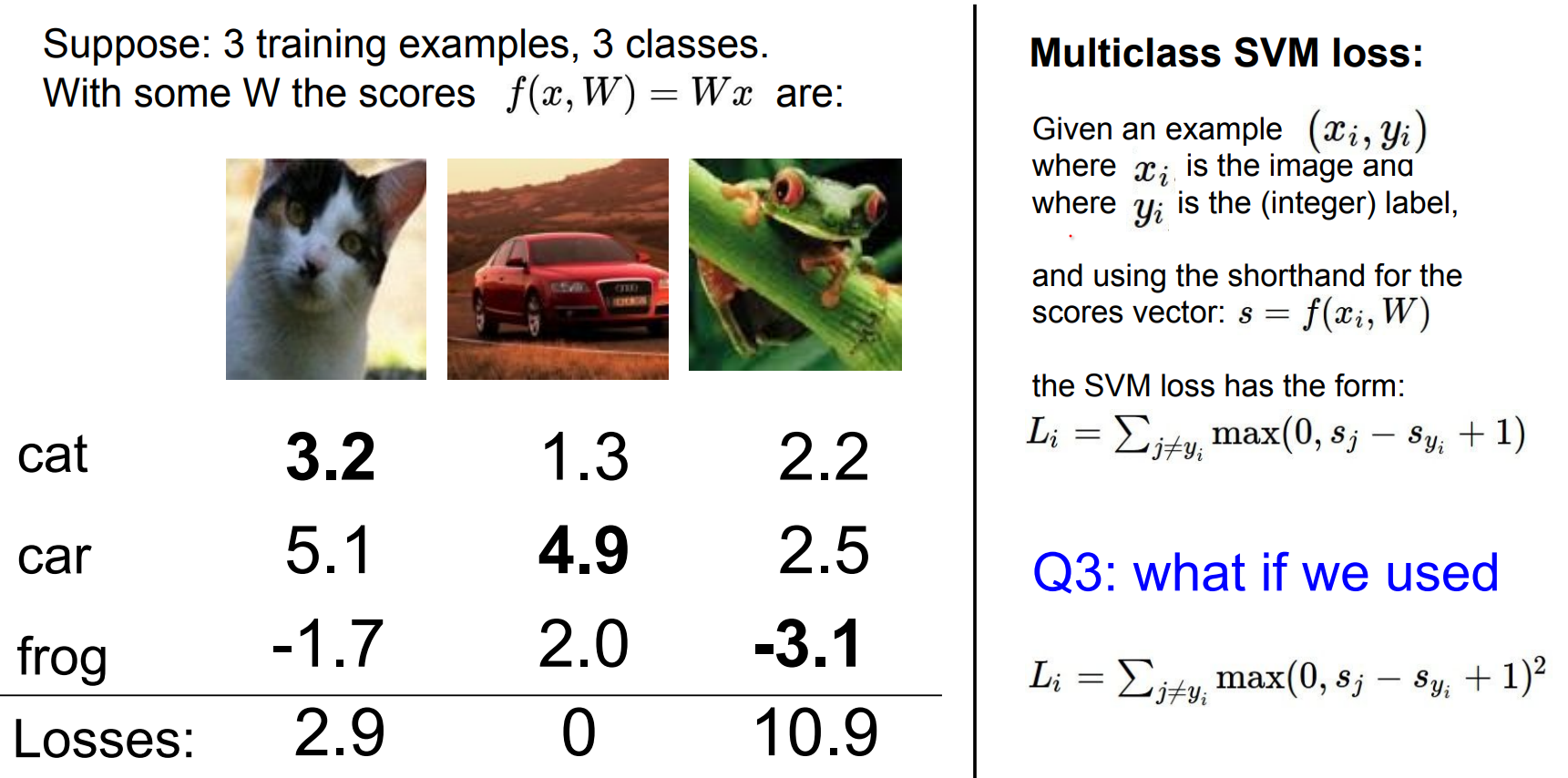
• Can we use a different penalty?
  We would get a different loss, because we are not just adding or removing a constant to the loss, we are changing the trade-off non linearly in different examples.

This is actually called Squared Hinge Loss. This is a hyperparameter and sometimes it works better.

Squared hinge loss changes the trade-off non-linearly and can behave better or worse depending on the dataset.

• What are the min/max losses?
  Minimum is 0, maximum is unbounded.

• What loss should we see at random initialization (scores ~ 0)?
  Another way of asking this is that usually at initialization \(W\) are small numbers, so all \(s ~= 0\). What is the loss?

Expect roughly (number_of_classes - 1) as a sanity check.

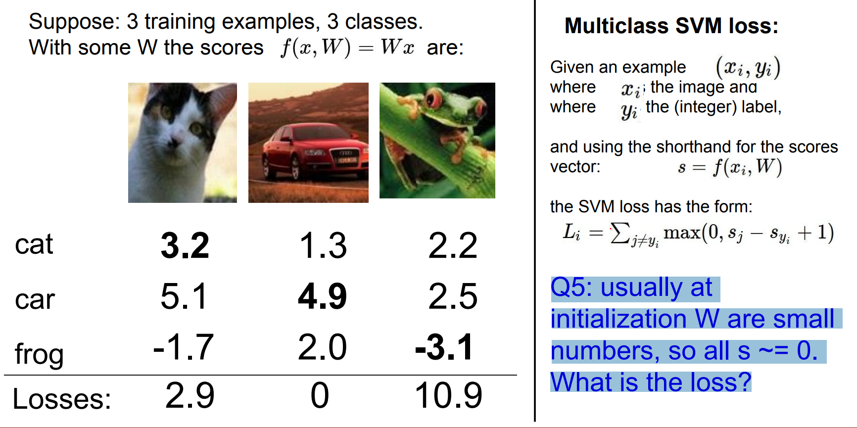
Using this loss, Your first loss should be number_of_classes - 1. This is important for sanity checks.

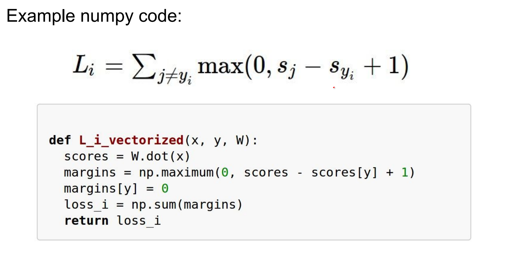
def L_i_vertorized(x, y, W):
    """
    X is a single colmun vector 
    y is class of the image (integer)
    W is weight matrix

    """
    scores = W.dot(x)
    margins = np.maximum(0, scores - scores[y] + 1)
    margins[y] = 0
    loss_i = np.sum(margins)
    return loss_i

In open form we got this:

Why Regularize?

Even if multiple weight matrices produce zero data loss, we prefer ones with "nicer" properties (e.g., small weights, smoother decision boundaries).

This is not really obvious.

E.g. Suppose that we found a \(W\) such that \(L = 0\). Is this W unique? Is there a W that is different but achieves zero loss.

Actually there could be a lot of \(W\)'s giving us 0 loss. Here is an example:

We have this entire subspace of W's and it all works the same according to our loss function. We would like to have some W's over others, based on some things we want about W (forget the data).

• Regularization measures the niceness of your w.

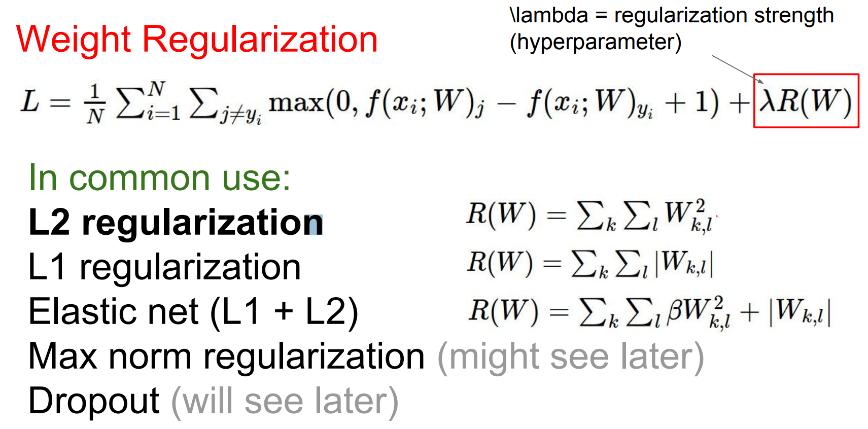
Regularization is a set of techniques where we are adding objectives to the loss, which will be fighting with the part where the loss is just want to fit to the data, because we want both of them.

Even if the training error is worse (we are not correctly classifying all examples), test set performance is better with these regularization's.

Most common is L2 Regularization - Weight Decay.

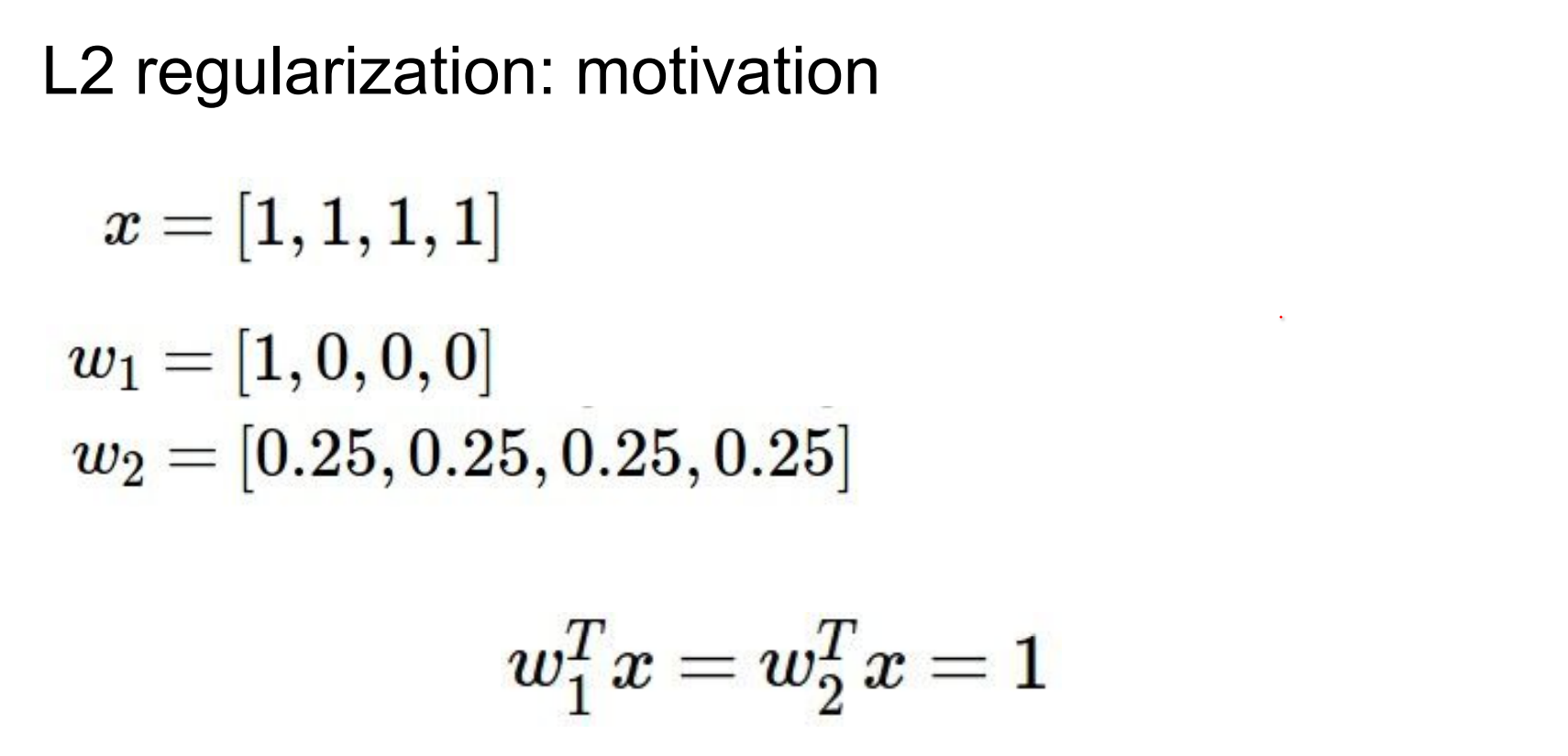
The effect of these w's are the same. We want low w's across board (diffused weights) if possible.

But regularization will strictly favor one of them.

Second one is way better. Why? It takes into account the most things (dimensions) in your input vector X. Our Losses will always have these.

• Most commonly used two linear classifiers: SVM - Softmax Classifier (Multinomial Logistic Regression) 🤔

Every loss we use in practice will be "data term + regularizer."

Softmax / Multinomial Logistic Regression

The softmax function is named as such because it is a "soft" or smooth version of the maximum function (argmax).

It takes a vector of arbitrary real-valued scores and transforms them into a probability distribution over multiple classes.

It does this by exponentiating each score and then normalizing the results by dividing by the sum of the exponentiated scores.

This normalization ensures that the output values fall between 0 and 1 and sum up to 1, making them interpretable as probabilities.

The softmax is a smooth approximation to argmax. It turns raw scores into probabilities by exponentiating and normalizing.

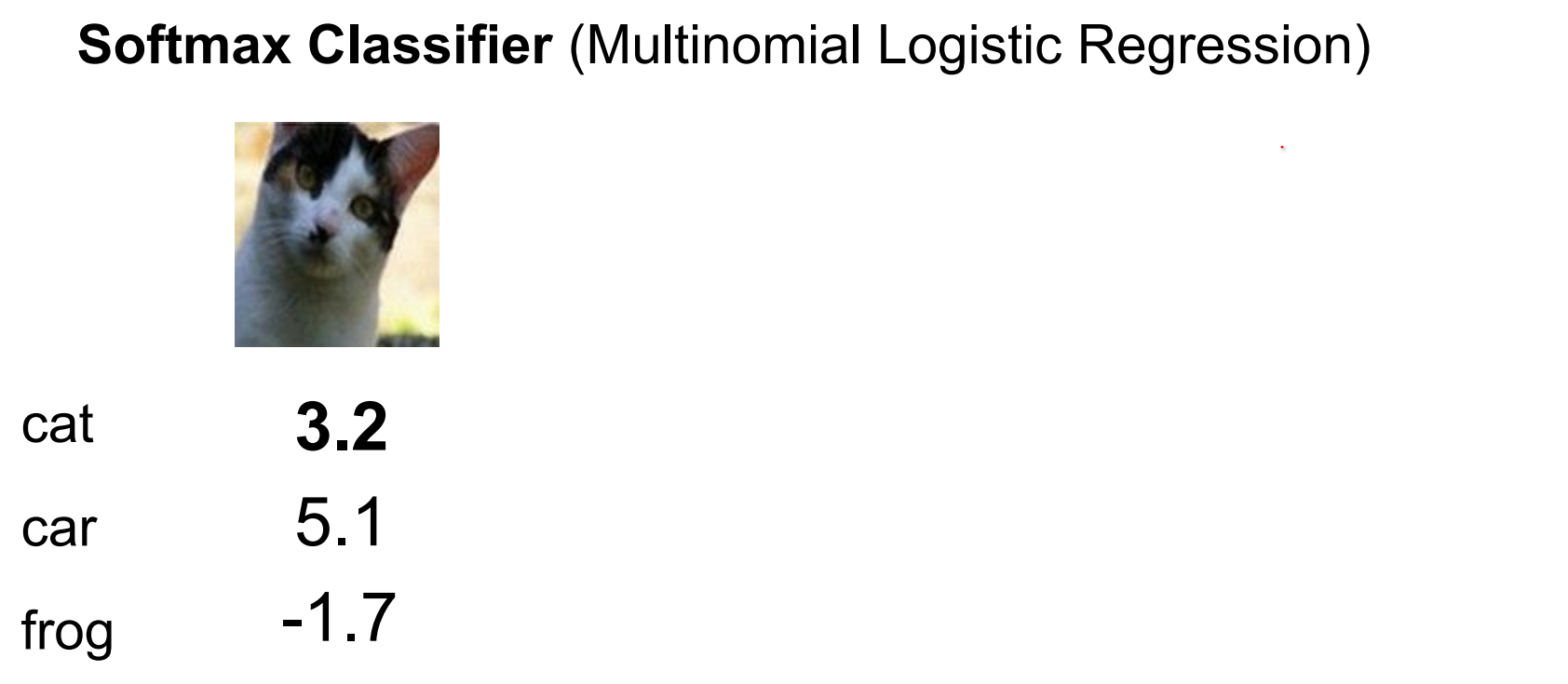
This is just a generalization of Logistic Regression. 🤔

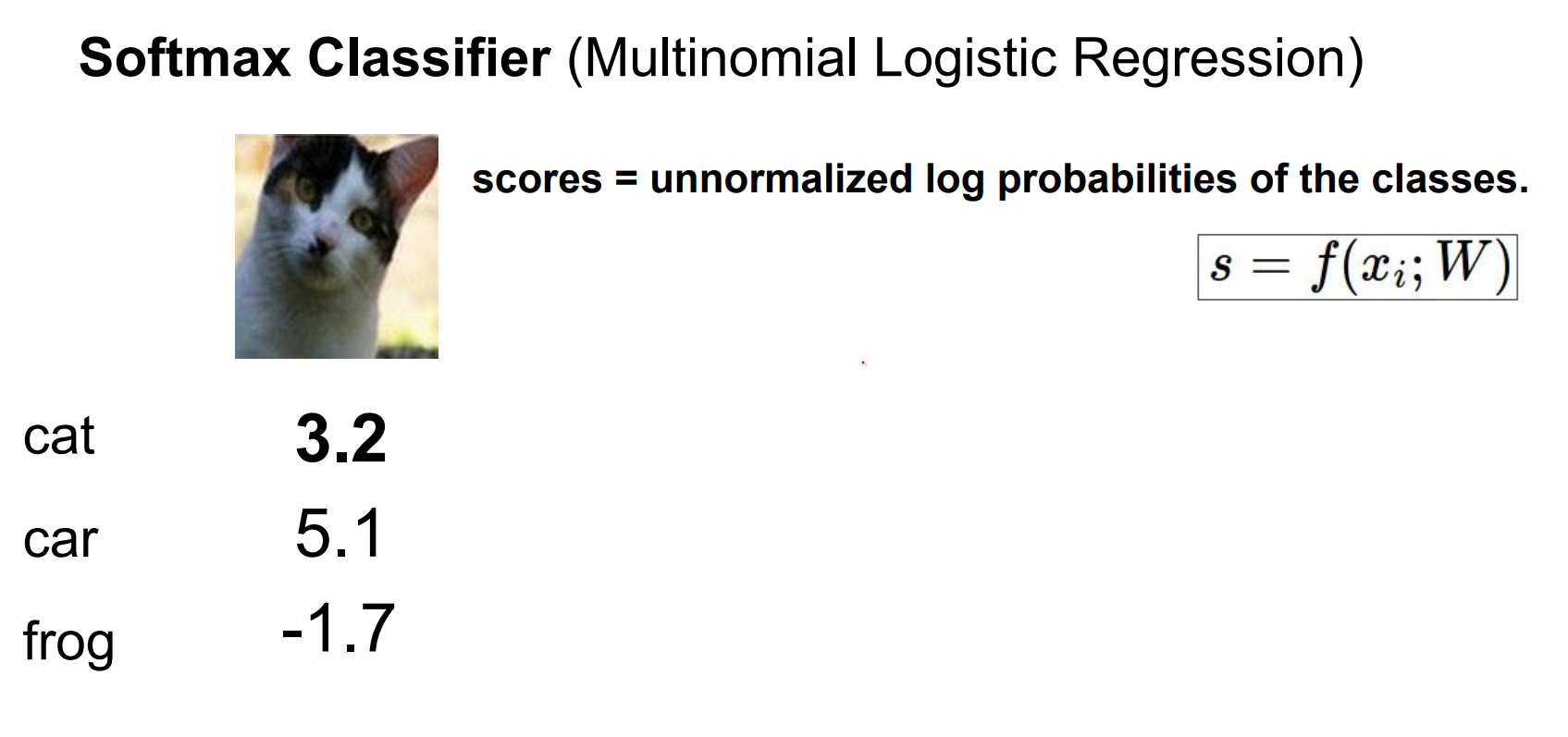
These are scores: unnormalized log probabilities.

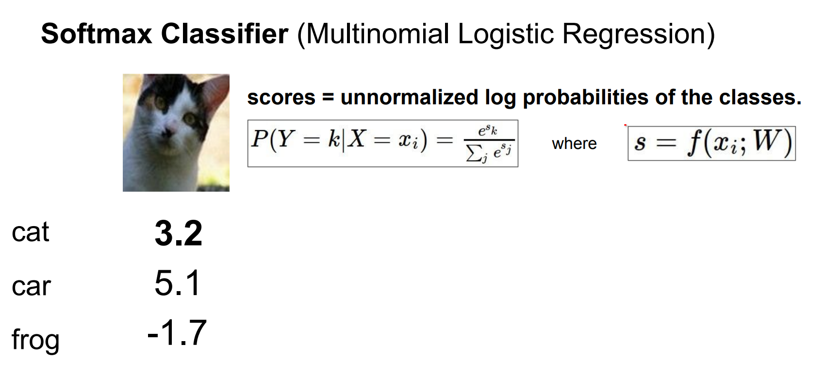
The way to get probabilities of different classes, like class k - \(Y = k\)

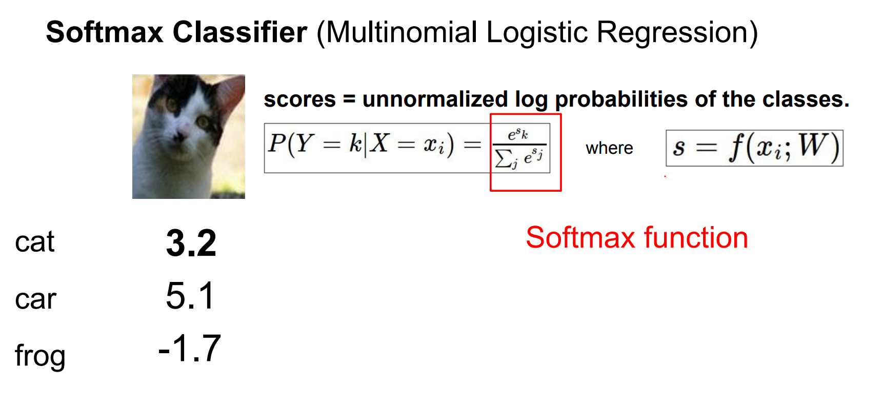
We take the score, we exponentiate all of them to get the unnormalized probabilities, and we normalize them. This is the softmax function.

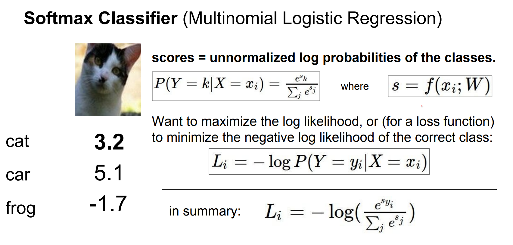
We want the log likelihood of the correct class to be high. The log likelihood is the softmax of your scores. Lets see an example.

From Scores to Probabilities

1. Compute class scores \(f_k\).
2. Exponentiate to obtain unnormalized probabilities.
3. Normalize by dividing through the sum so outputs are in (0,1) and sum to 1.
4. Use the negative log-likelihood of the correct class as the loss.

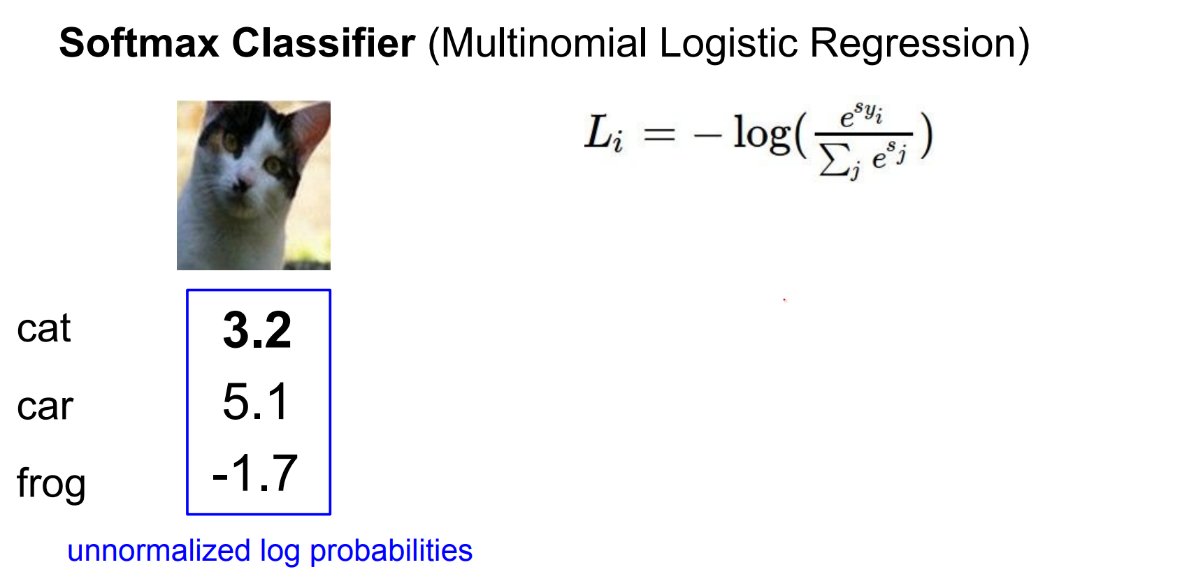
This came from our classifier.

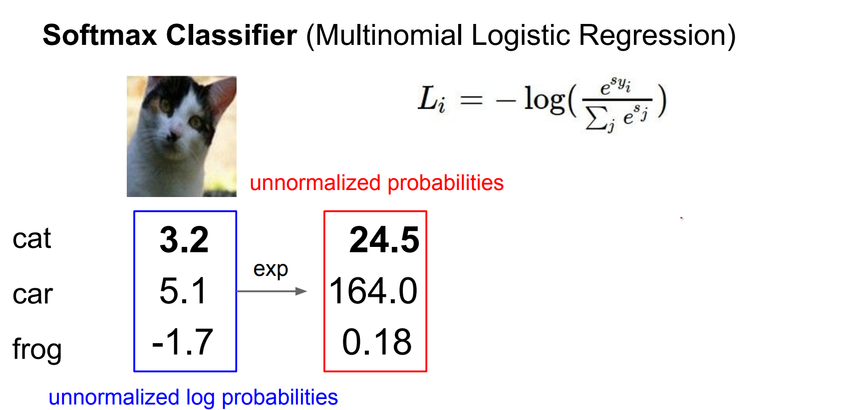
We exponentiate them first.

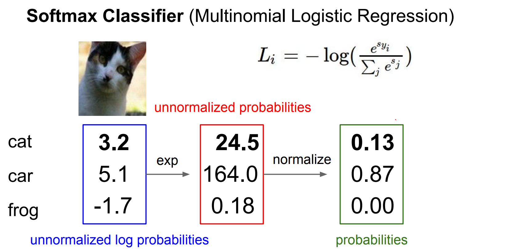
Probabilities always sum to 1, so we want to divide these.

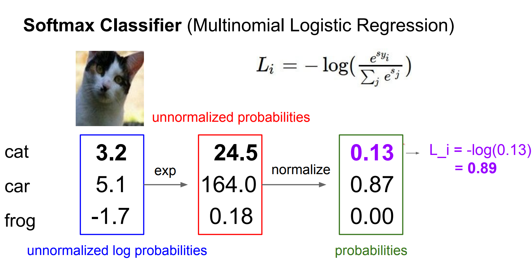
In final we found 0.89 for Cat. The example assigns 0.89 probability to "cat" after normalization.

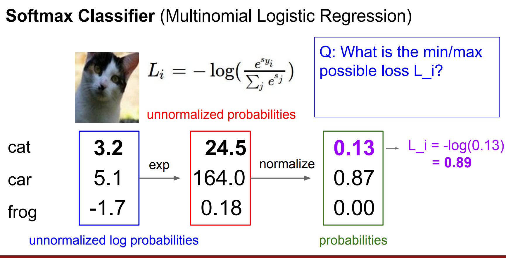
Softmax Sanity Checks

• Minimum loss is 0; maximum is unbounded. Min value - 0 / highest possible is infinity.

• With tiny random weights (scores ~ 0), the initial loss should be \(\(-log(number_of_classes)\)\).

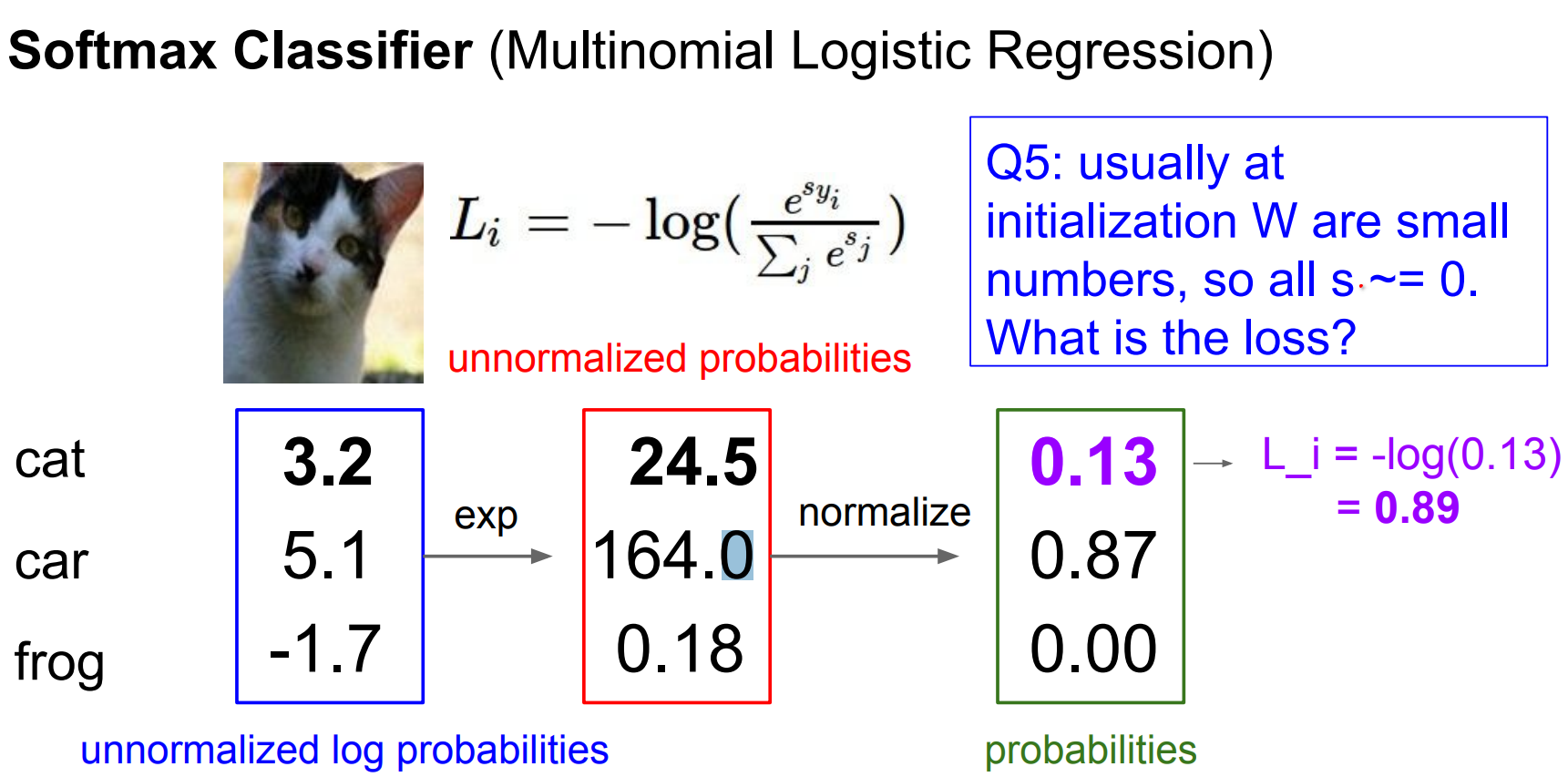
Tangent - Insight Checklist

• Note the number of classes.
• Compute -log(K) and confirm the initial loss matches.
• Aim to drive the loss toward 0; it will never go negative.

Here is the summary so far.

We had Hinge loss, where we used scores directly with our loss function. We just want the correct class score to be some margin above the other classes.

With Softmax loss, we use unnormalized probabilities and normalize them and we want to maximize the probability of correct classes (over the log of them).

Why log? Log is a monotonic function. Maximize a probability is exactly the same for maximizing the logarithmic probability. Log is much nicer in math.

• They start of the same way but different approaches. In practice when you run the two, gives almost the same result.

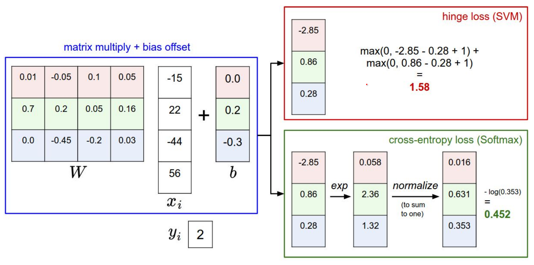
Hinge vs Softmax Comparison

• Hinge loss only cares about margins; once they are satisfied, small perturbations do nothing.
• Softmax keeps pushing scores so that probabilities concentrate on the correct class.
• Logs are monotonic, so maximizing probability equals maximizing log-probability, but logs yield nicer math and gradients.

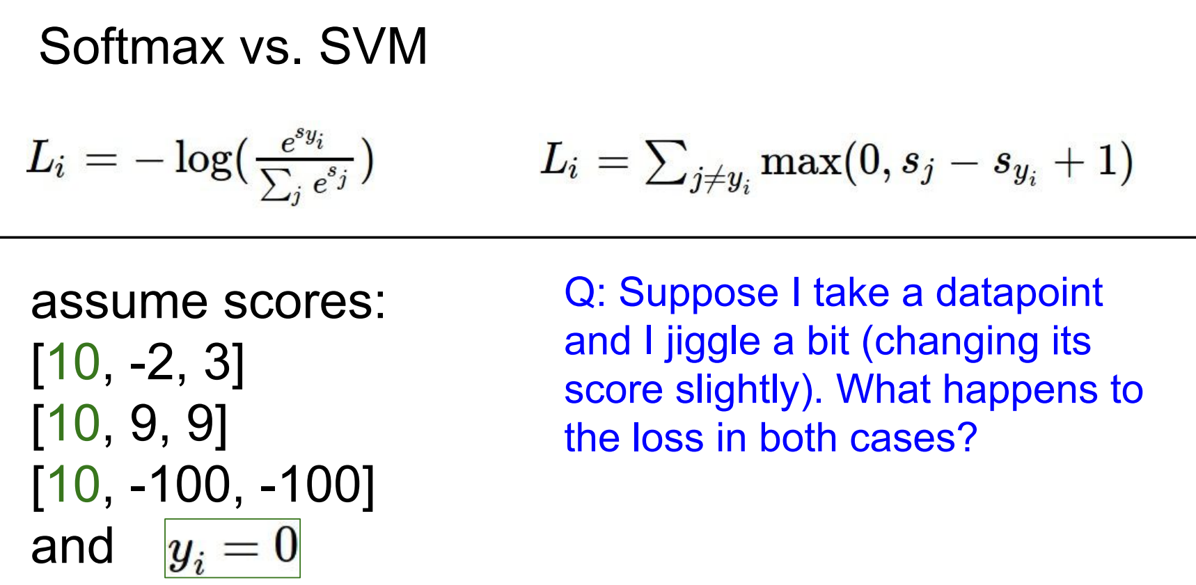
Green is the correct classes.

If you jiggle a datapoint (Suppose I take a datapoint and I jiggle a bit (changing its score slightly). What happens to the loss in both cases?):

• SVM often ignores it once margins are satisfied.
• Softmax reacts immediately because probabilities change everywhere.

SVM is already happy, when we jiggle, it does not care. But Softmax would care a lot, it want the score at some specific ranges.

You are in charge of the loss function, if it is differentiable, you can write your own.

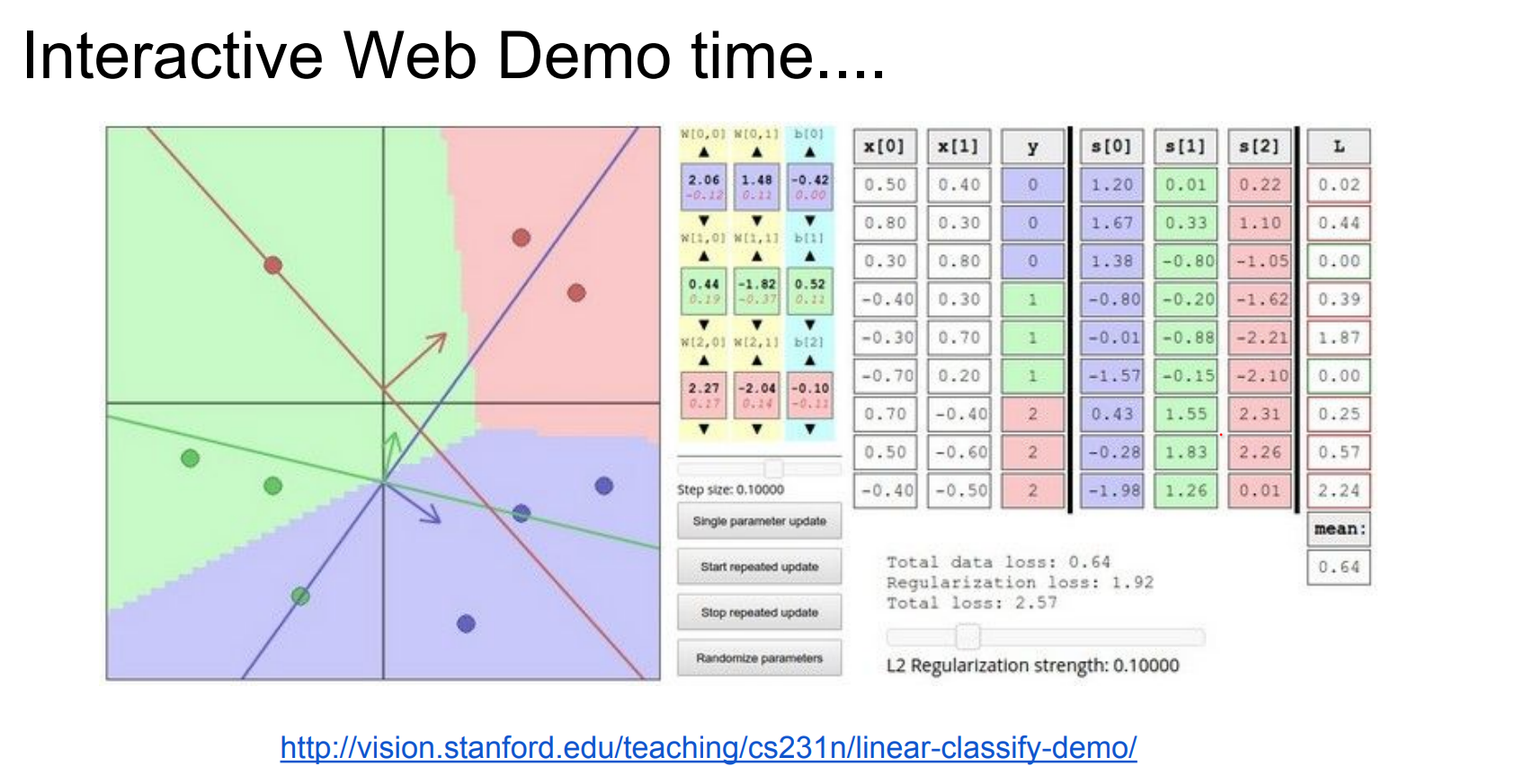
Try the interactive demo to see how different losses reshape W.

We can improve the set of W's we have. The total loss is decreasing.

At the start, we will use big step size, overtime, we will update the update size.

The class scores for linear classifiers are computed as \(f(xi;W,b)=Wxi+b\), where the parameters consist of weights \(W\) and biases \(b\) . The training data is \(x_i\) with labels \(y_i\).

In this demo, the data-points \(x_i\) are 2-dimensional and there are 3 classes, so the weight matrix is of size [3 x 2] and the bias vector is of size [3 x 1].

The multi-class loss function can be formulated in many ways. The default in this demo is an SVM that follows [Weston and Watkins 1999].

---

Optimization

Optimizers are responsible for minimizing the loss function by adjusting the model's parameters, while regularization techniques modify the loss function to encourage simpler solutions and prevent overfitting.

These components work together to train effective machine learning models.

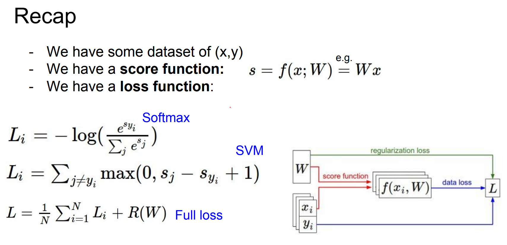
Summary of the information flow. The dataset of pairs of (x,y) is given and fixed. The weights start out as random numbers and can change. During the forward pass the score function computes class scores, stored in vector f.

The loss functions contains two components 💙

• The data loss computes the compatibility between the scores f and the labels y.

• The regularization loss is only a function of the weights.

During Gradient Descent, we compute the gradient on the weights (and optionally on data if we wish) and use them to perform a parameter update during Gradient Descent.

Better W is a smaller loss.

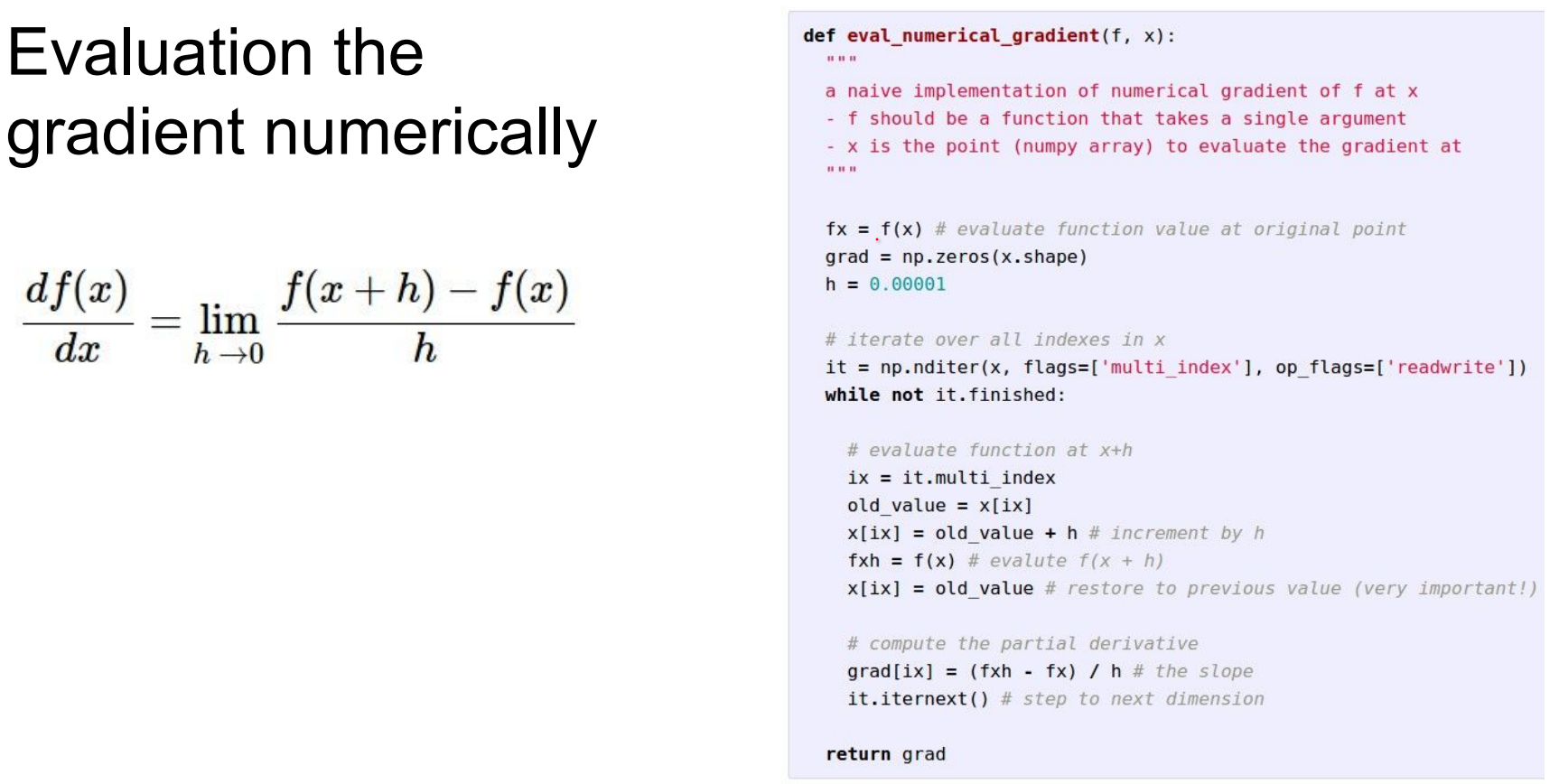
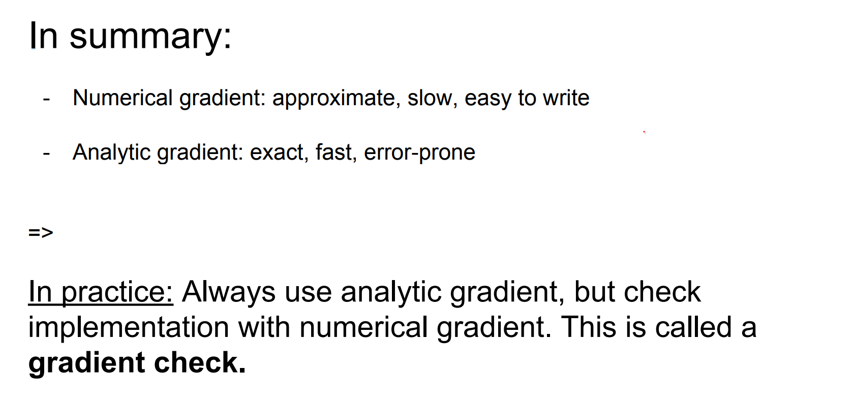
Numerical vs Analytic Gradients

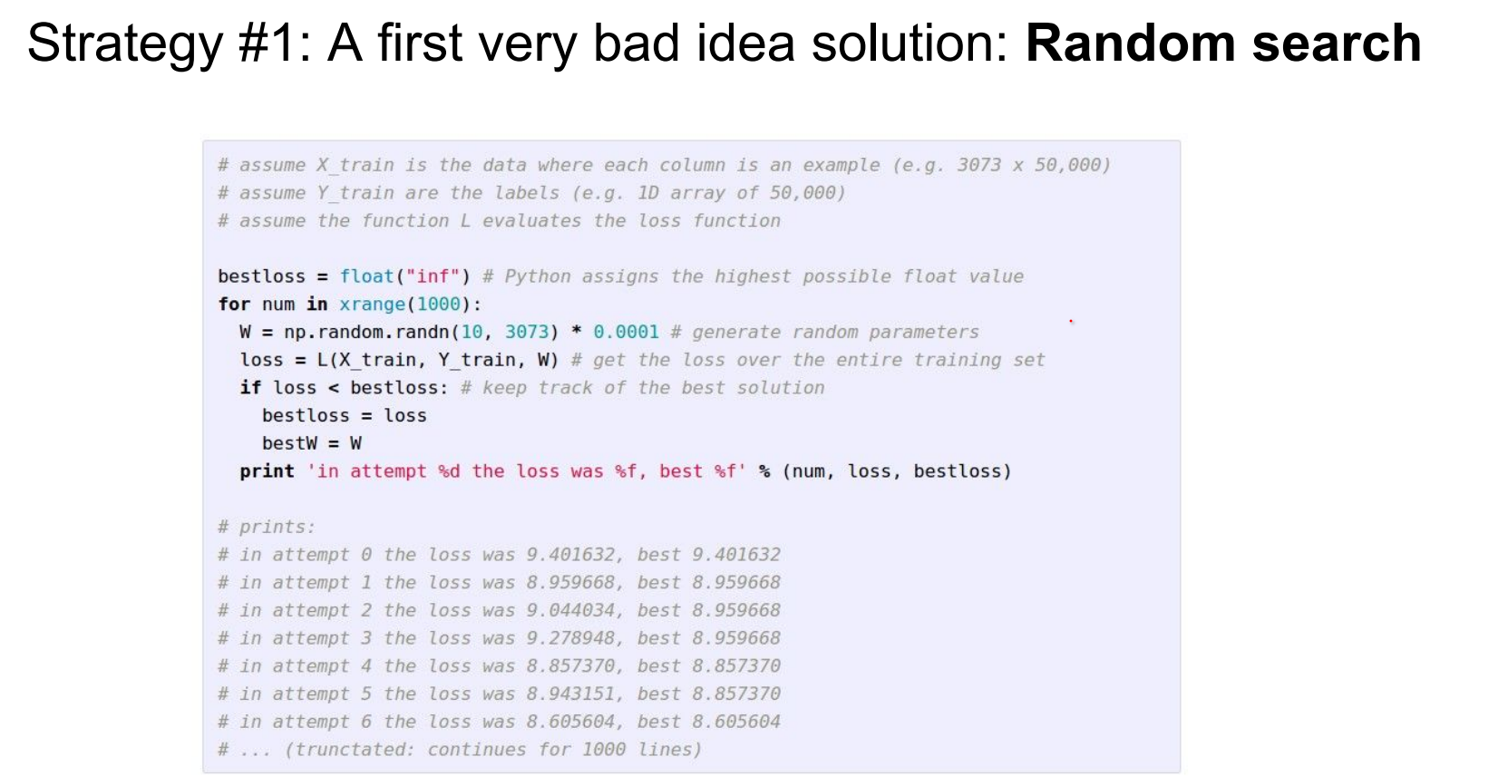
Blind "teleport-and-measure" searches are hopeless in high dimensions. Slide 3037 shows the brute-force intuition: try a random direction, move slightly, measure the loss. Do that in millions of dimensions and you are doomed.

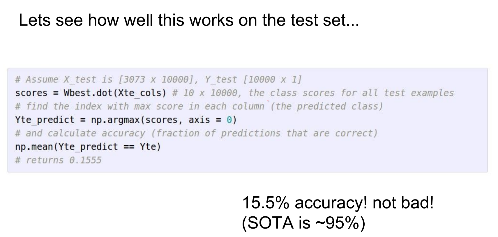
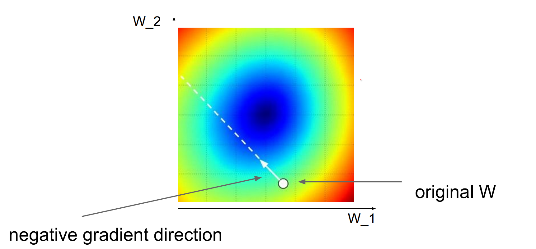
You have an altitude meter and blindfolded.

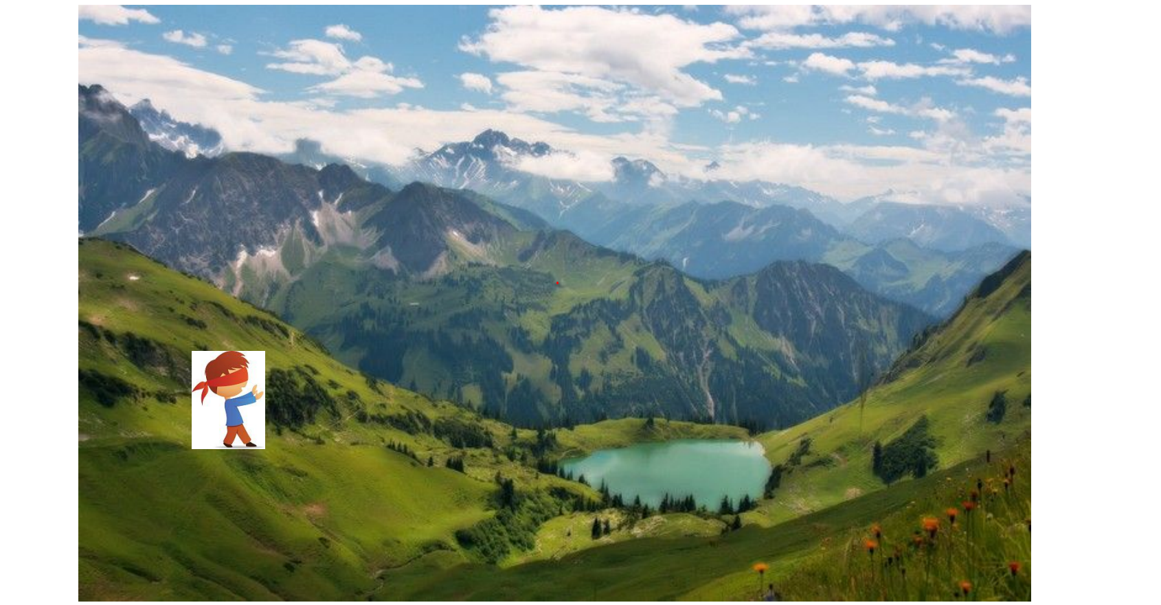
Instead of teleporting different places and read altitude, compute slope and go downhill.

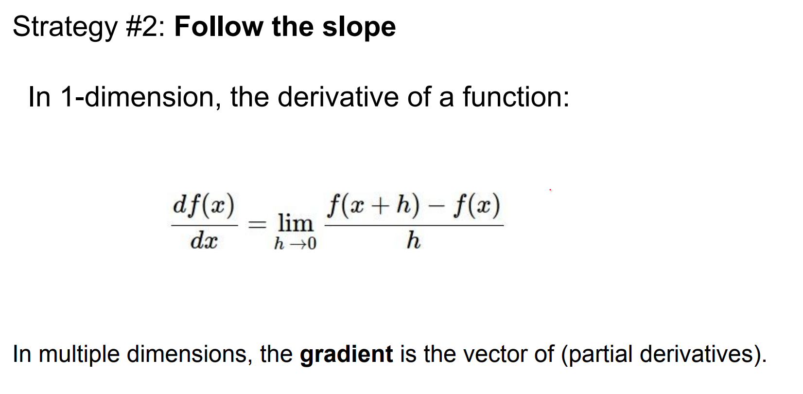
We have multiple dimensions, multiple W's so we have a gradient.

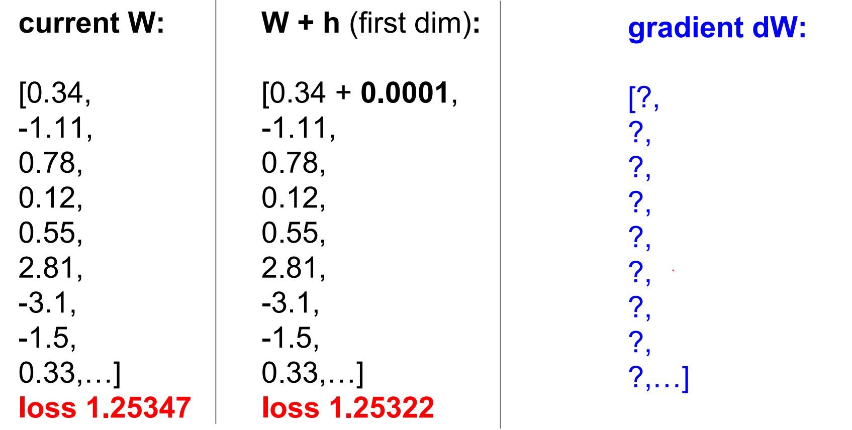
• Gradients give the slope; evaluate f(x + h) and f(x - h) to estimate it. This is just the definition of a derivative written as a finite difference.
• Repeat for every dimension to know which way is downhill. With D parameters you need to do 2D forward passes just to get a direction—ouch.

def numerical_grad(f, x, h=1e-5):
    grad = np.zeros_like(x)
    for i in range(x.size):
        old_val = x[i]
        x[i] = old_val + h
        fxph = f(x)
        x[i] = old_val - h
        fxmh = f(x)
        grad[i] = (fxph - fxmh) / (2 * h)
        x[i] = old_val
    return grad

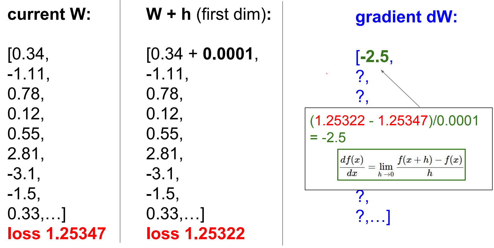
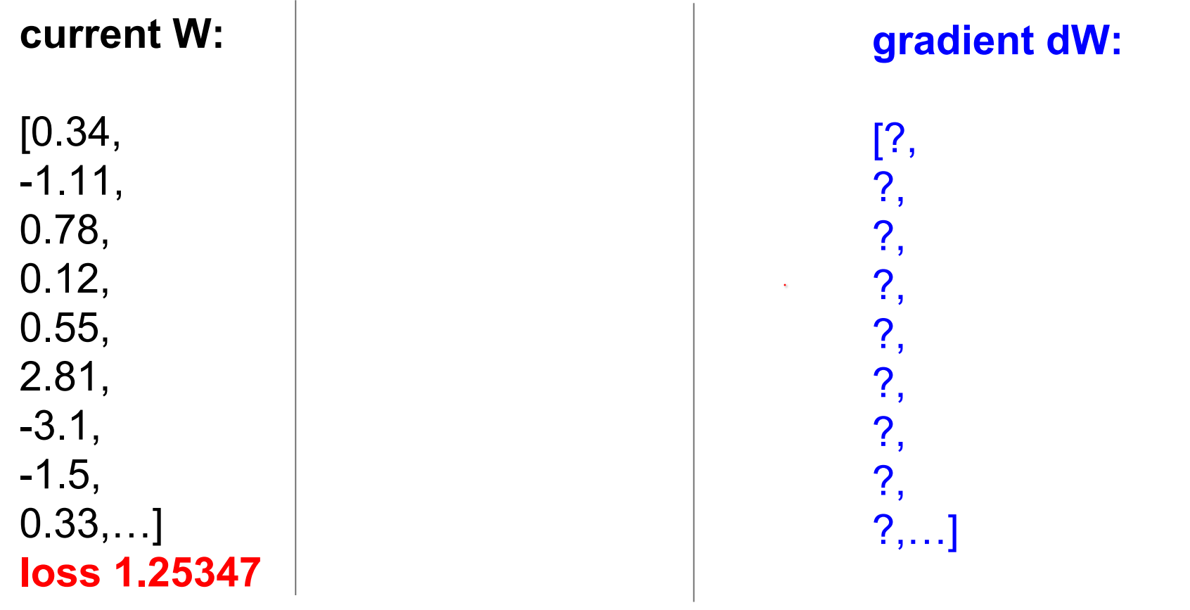
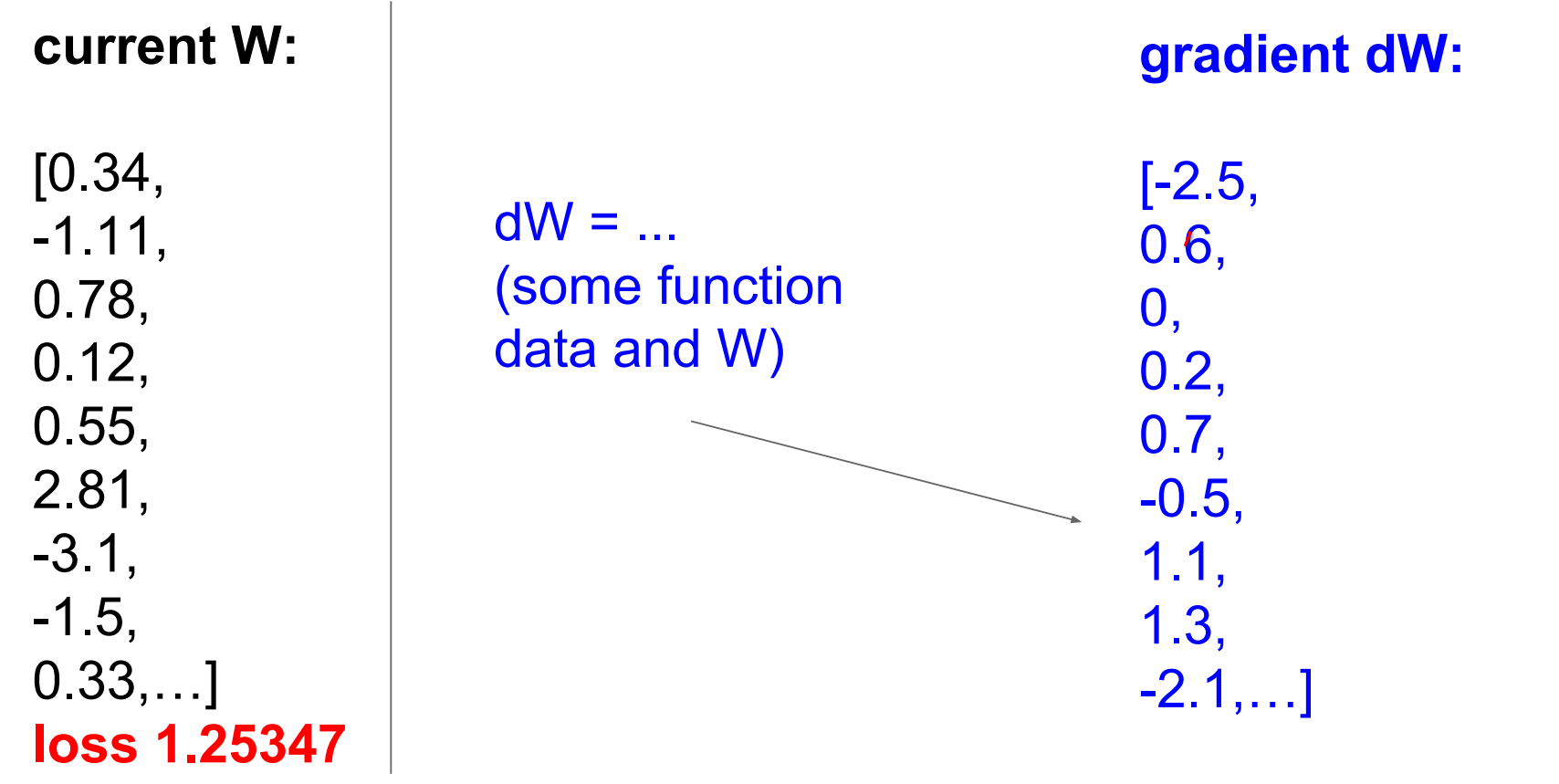
SO the gradient is -2.5 I took a step and it worked!

DO this for every dimension.

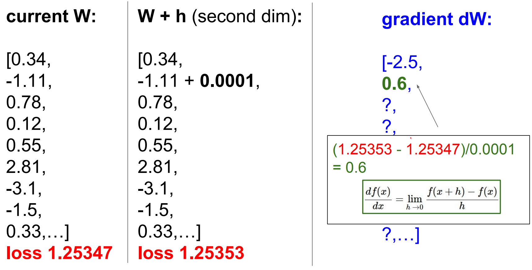
And another one.

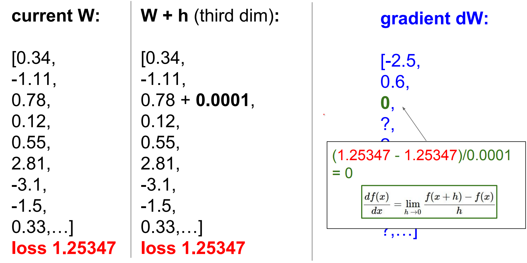
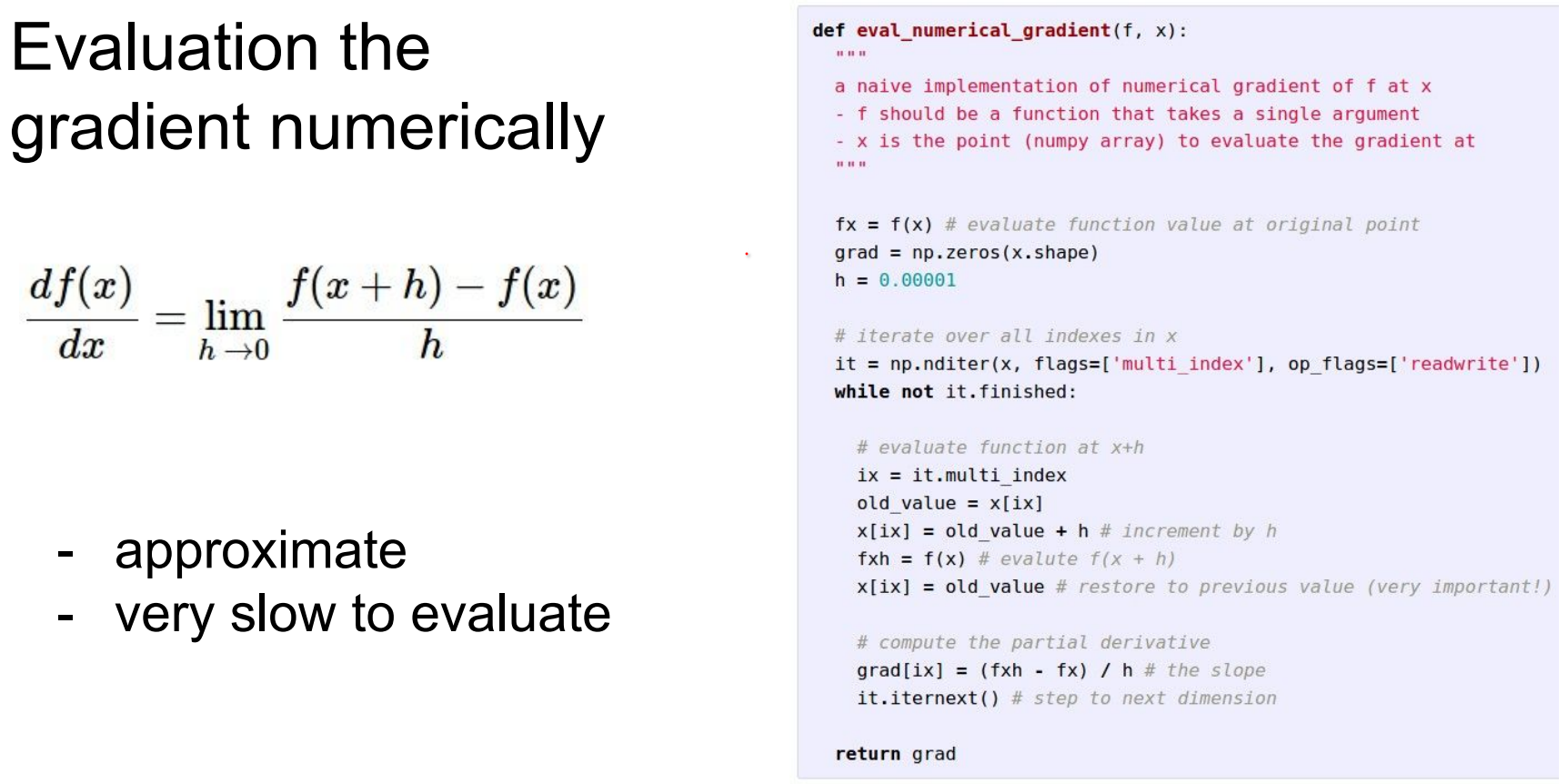
Most basic way:

This is very slow we have million of parameters.

We cannot check millions of parameters before we do a single step. 😕

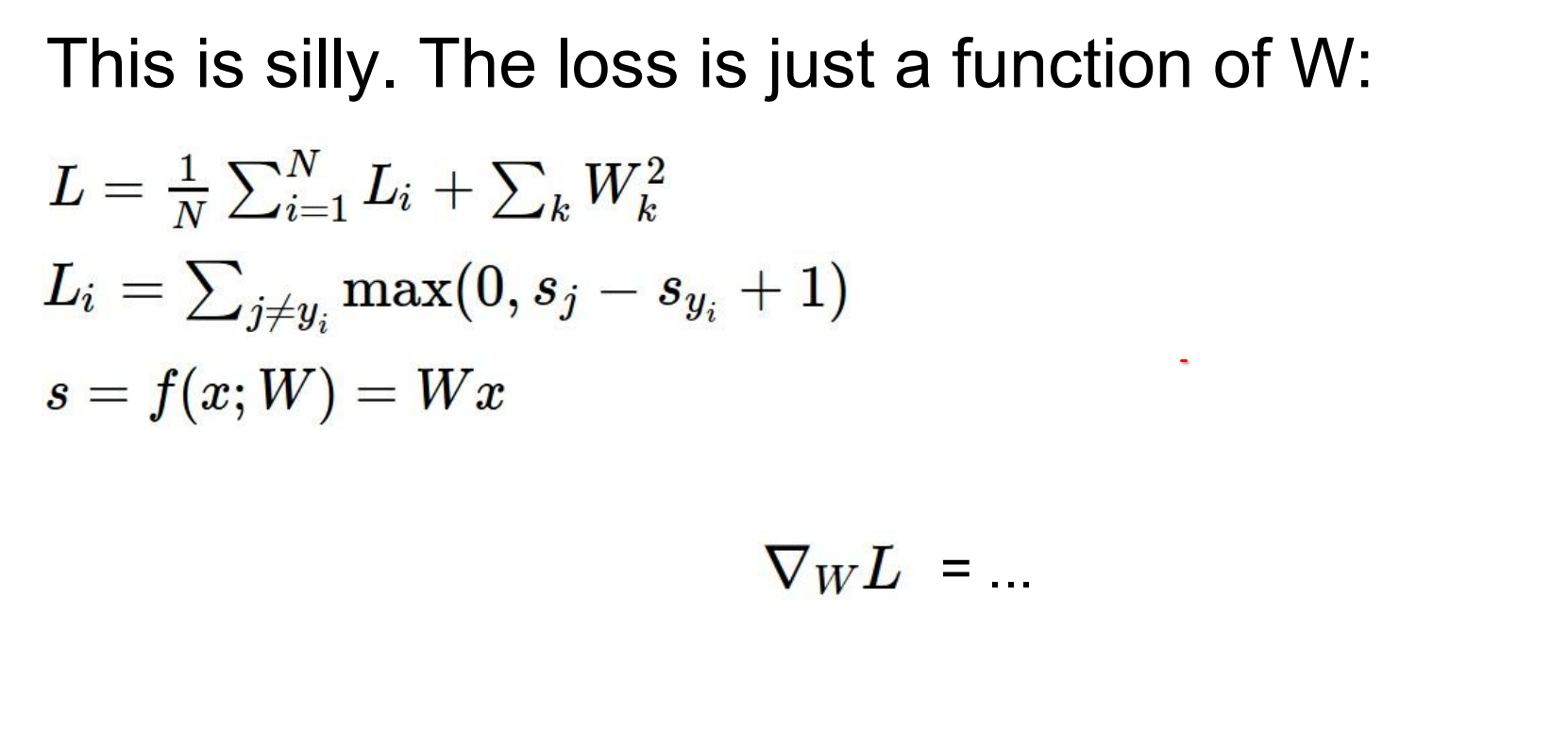
This is silly. The loss is just a function of W, we want the gradient of the loss function wrt W.

We can just write that down.

In other words, instead, derive gradients analytically with calculus. Once we know how the loss is composed from operations (matrix multiply → max → sum, etc.) we can back-propagate derivatives with the chain rule in one forward/backward sweep.

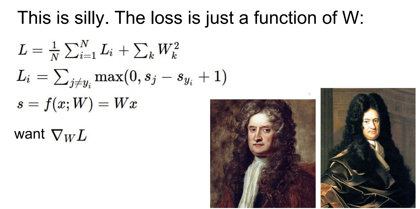
Newton and Leibniz. They actually found Calculus. There is actually controversy over it.

Instead of evaluating numerical gradient, we can use calculus write than expression of what the gradient is of that loss function in weight space.

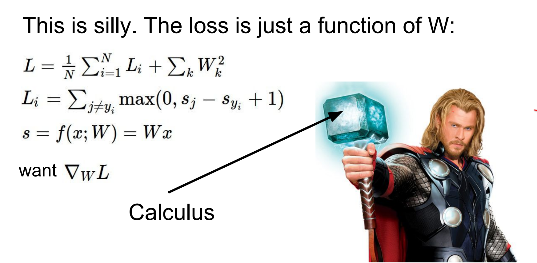
In practice, always use analytic gradients but confirm correctness with a numerical gradient check. Think of it as a unit test: run once per new layer, compare numbers, and only then trust the fast analytic path.

Step Size / Learning Rate is the most critical Hyper-parameter that you will work on.

Gradient Descent Loop

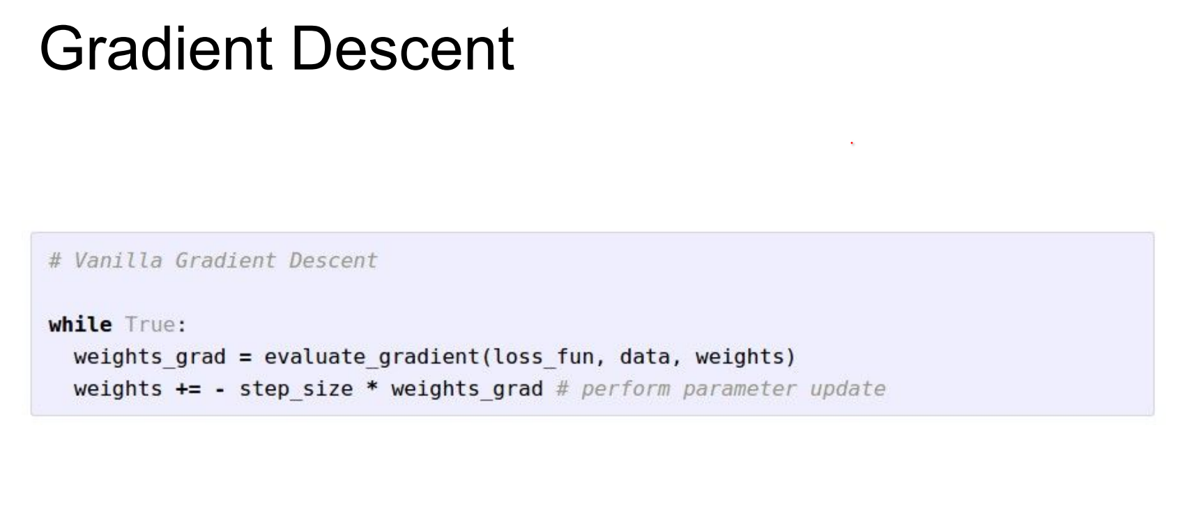
• Compute gradients of the loss with respect to weights: forward pass for scores, loss, backward pass for dW.
• Update W by stepping opposite the gradient (-learning_rate * grad). One line of numpy changes the entire classifier.
• Learning rate (step size) and weight regularization are the most sensitive hyperparameters. Too high? Divergence. Too low? Snail pace.
• Keep iterating until loss plateaus.The classic pseudocode with a stopping condition based on iteration count or loss change.

Jump is high in red parts, blue parts are small.

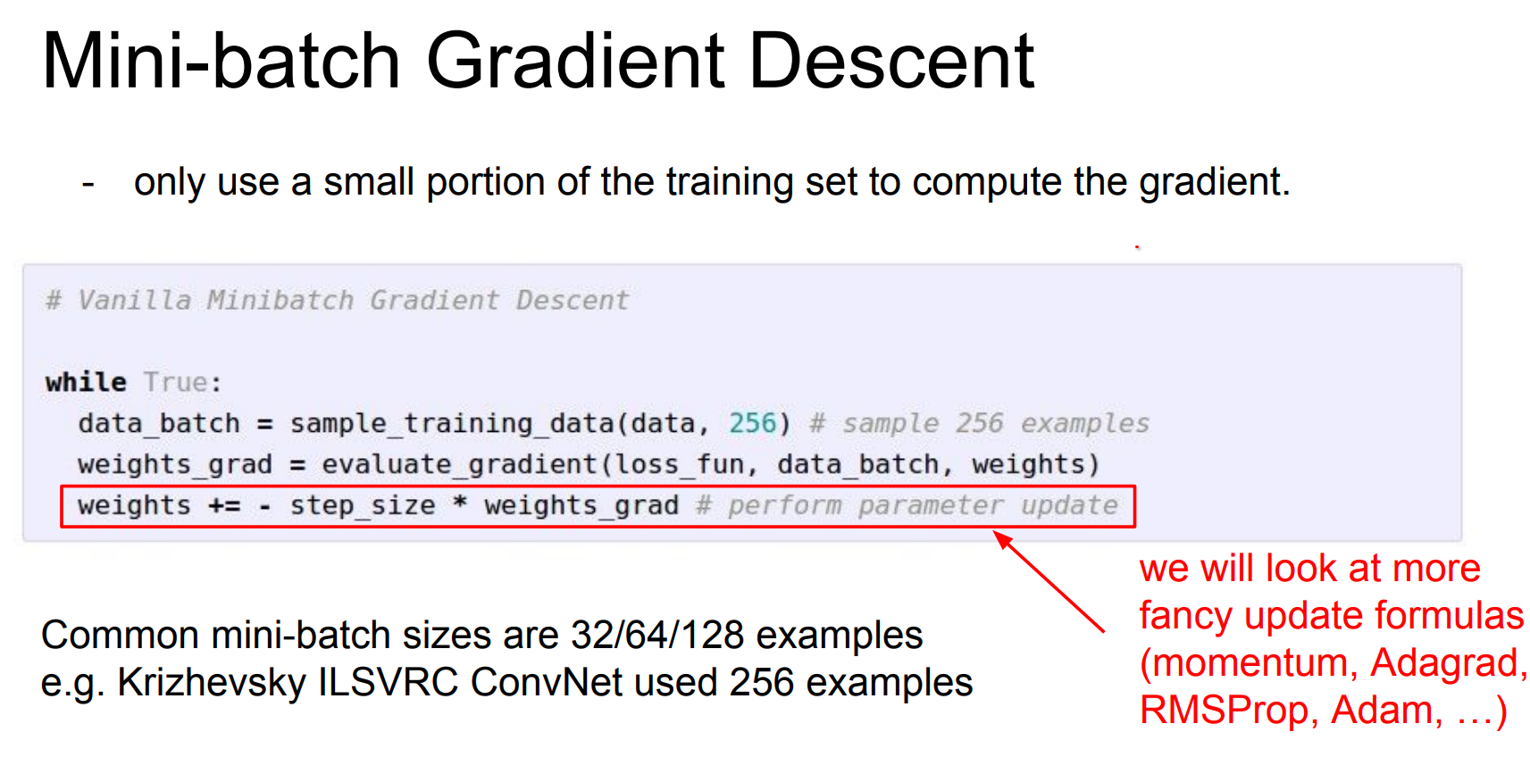
In Practice, we do not evaluate the loss of the entire dataset, we sample batches from the data.

Mini-batches and Noise

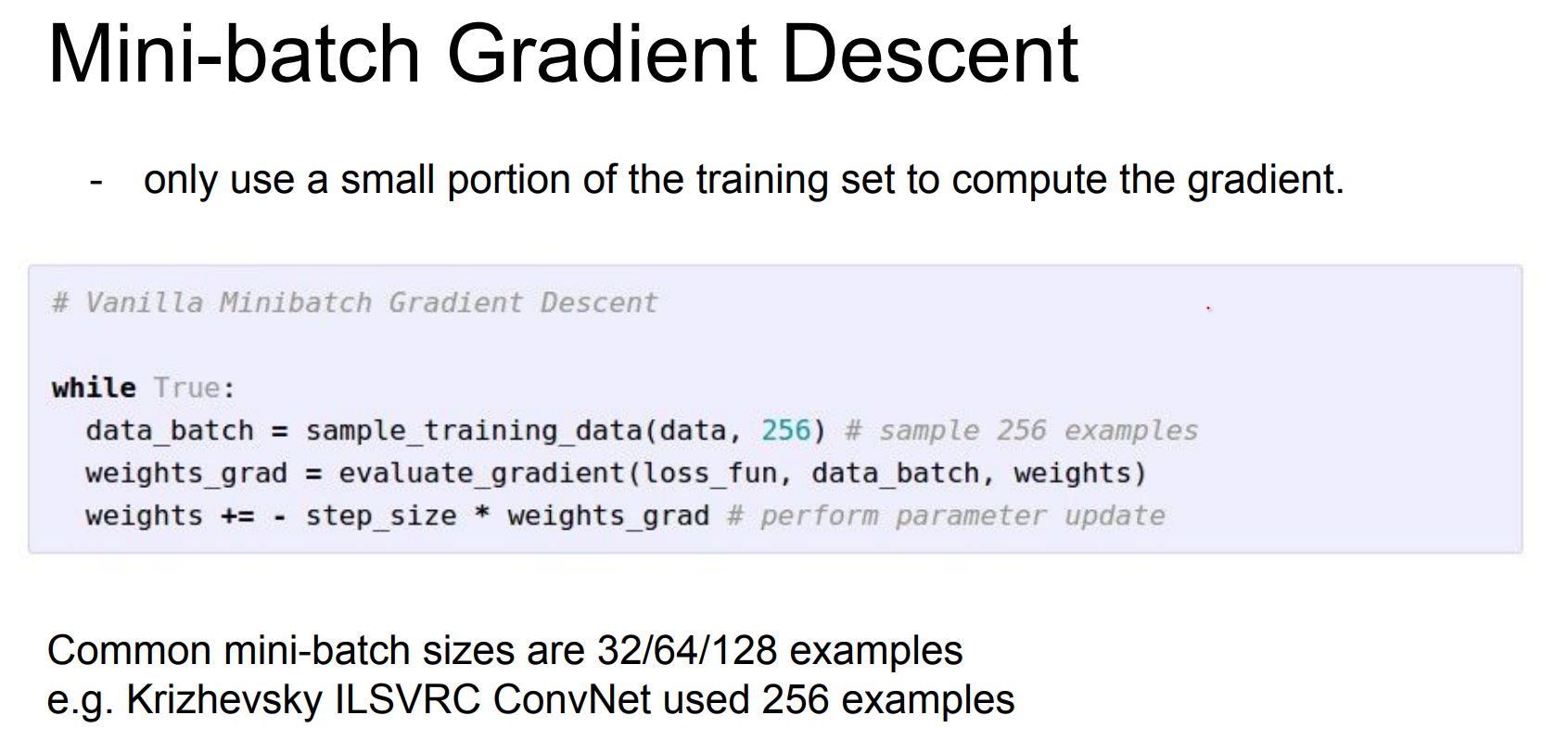
• Full-dataset gradients are expensive; we use stochastic (mini-batch) estimates instead. Pick, say, 256 examples, approximate the gradient, update W, repeat with a new batch.
• Batch size is often dictated by GPU memory. On CPU you might use 32–128; on GPUs you go bigger until you run out of memory.
• Expect noisy, "wiggly" loss curves because of the sampling process. Slides 3054–3056 show the jagged training curves compared to the smooth full-batch line.
• This noise is not purely bad—it helps jump out of shallow local minima and acts as an implicit regularizer.

Much more efficient. Batch size is usually decided by GPU memory size.

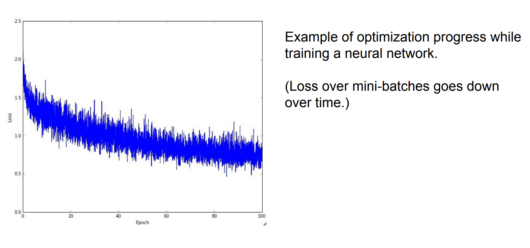This is what it looks like. Because we are using batches of data we have the wiggling.

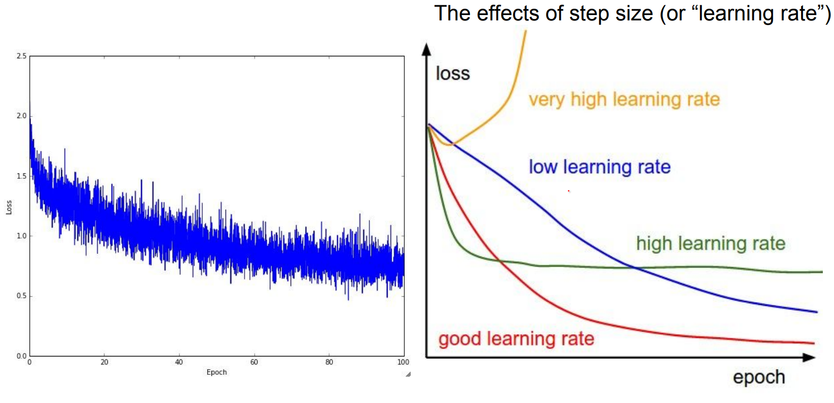
These are effects of learning rate.

Momentum and Variants

The way we do the update, how we used gradient to change w.

There is also momentum, where I also keep track of my velocity. Stochastic Gradient Descent with Momentum.

• Vanilla SGD updates use only the current gradient; think of it as a ball that instantly stops after each move.
• Momentum keeps track of velocity: v = μ v - η grad; W += v. The previous direction influences the next, helping the ball roll through shallow valleys instead of jittering.
• Nesterov momentum (look ahead before computing the gradient) is another tweak Andrej likes.
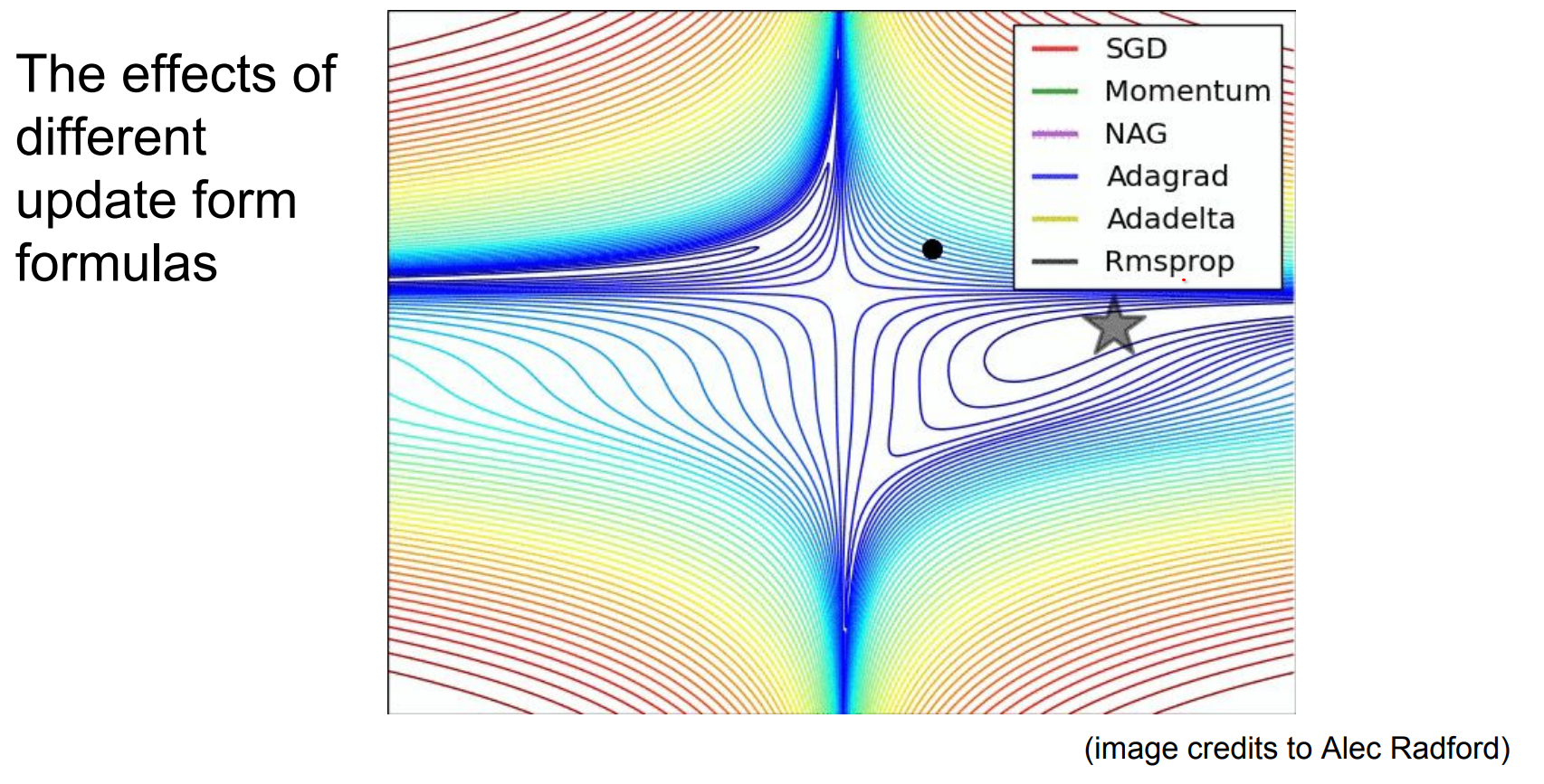
• Different optimizers (SGD, Adam, RMSprop, Adagrad) are all ways to update weights using gradient information plus extra heuristics such as adaptive learning rates per parameter.

Watch this GIF to see trajectories for various optimizers.

Optimizer, Loss, Regularization -- How They Interact

1. Loss functions (SVM, Softmax, MSE) quantify prediction error.
2. Regularizers (L1, L2, dropout, early stopping) discourage overfitting by penalizing model complexity.
3. Optimizers (SGD, Adam, RMSprop, Adagrad) navigate weight space using gradients of the (loss + regularizer).

Regularization modifies the loss surface, the optimizer follows the gradients on that surface, and the combination determines how well the model generalizes. Whenever training accuracy looks great but validation tanks, revisit this triangle: maybe the loss is wrong for the task, maybe λ is too small, maybe the optimizer needs a schedule tweak.

Feature Engineering Tangent

Before ConvNets dominated, we rarely fed raw pixels directly into linear classifiers. Instead, we engineered features and concatenated them into large vectors. The professional pipeline circa 2010 was: carefully craft statistics, pool them, then run a linear SVM. Andrej drops this tangent to remind us how luxurious end-to-end training feels now.

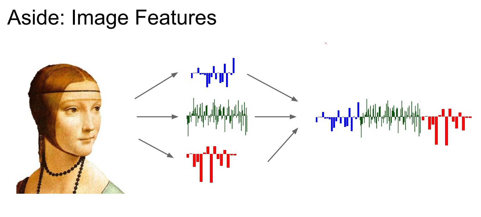
You do not want to put Linear Classifiers on pixels themselves, so you get different features.

And you can use the features to concatenate into big vectors and feed them into linear classifiers.

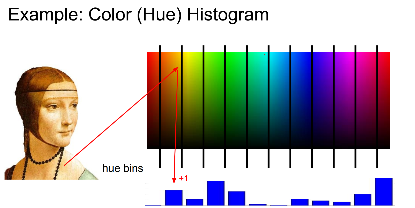
One simple feature type is a color histogram.

Go over of each pixel in image, bin them 12 for different colors depending on the Hue of the color.

This would be one of the features that we will be using with different feature types together.

Color Histograms and Hue

The color can be characterized by the following properties:

• hue: the dominant color, name of the color itself e.g. red, yellow, green.
• saturation or chroma: how pure is the color, the dominance of hue in color, purity, strength, intensity, intense vs dull.

• brightness or value: how bright or illuminated the color is, black vs white, dark vs light.

• Build histograms over, say, 12 hue bins by iterating over every pixel. The output is an array counting how often each color range appears. Great for coarse scene cues (“lots of blue → sky?”).

• Hue/saturation/value define perceived color: hue is the dominant wavelength, saturation the purity, and value the brightness. Switching from RGB makes the histogram more robust to lighting.
• Concatenate histograms from different spatial regions (spatial pyramids) to keep rough layout information.

HOG and SIFT

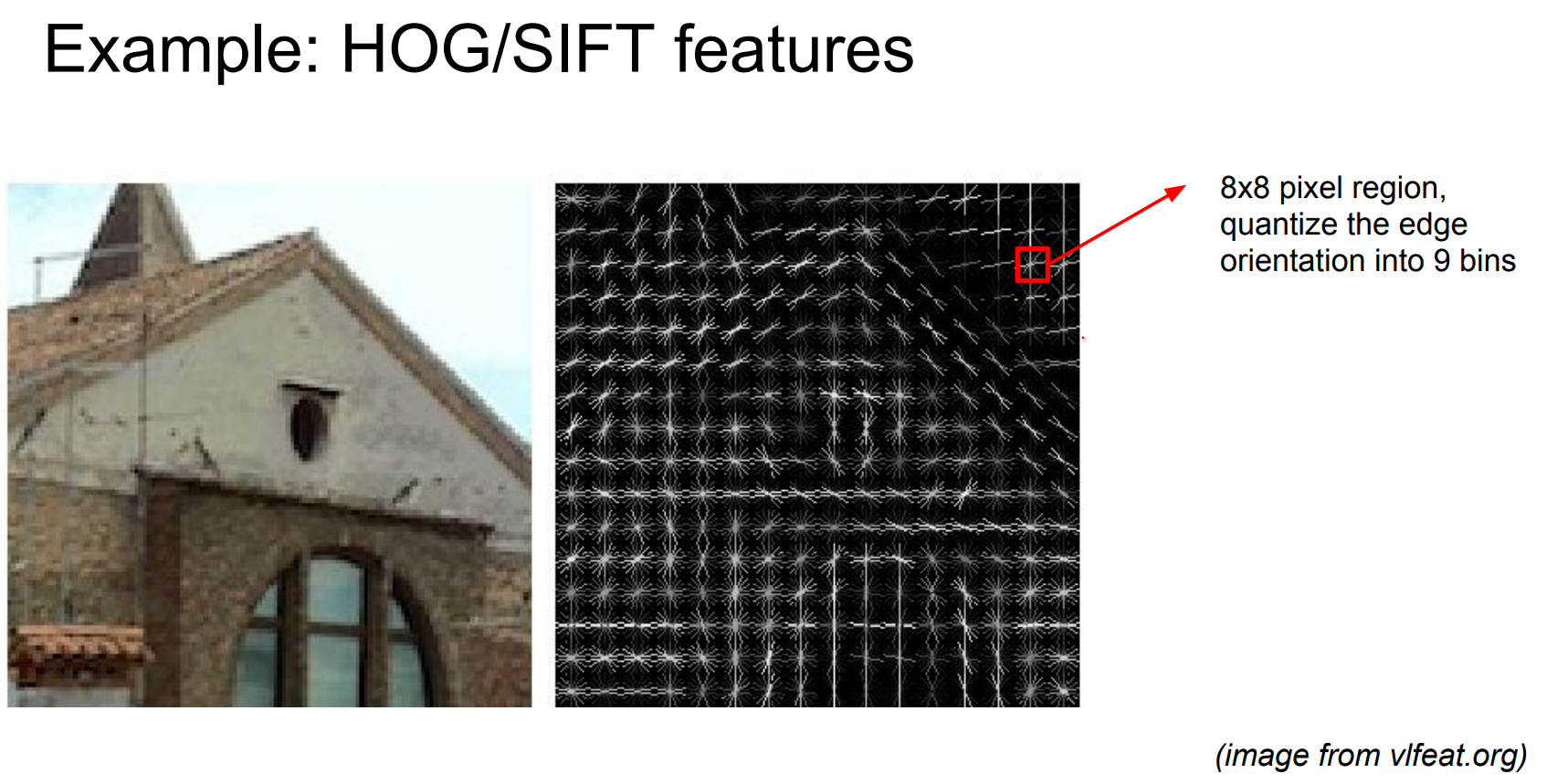
• Histogram of Oriented Gradients (HOG) divides the image into cells, computes x/y gradients, and accumulates orientations into bins. Blocks of neighboring cells get normalized and concatenated, producing a descriptor that says “there is a vertical edge here, a corner there”.
• Scale-Invariant Feature Transform (SIFT) detects keypoints across scales (scale-space extrema), then constructs rotation/scale-invariant descriptors around each keypoint for matching and recognition. You can compare descriptors with cosine similarity and find repeated structures.

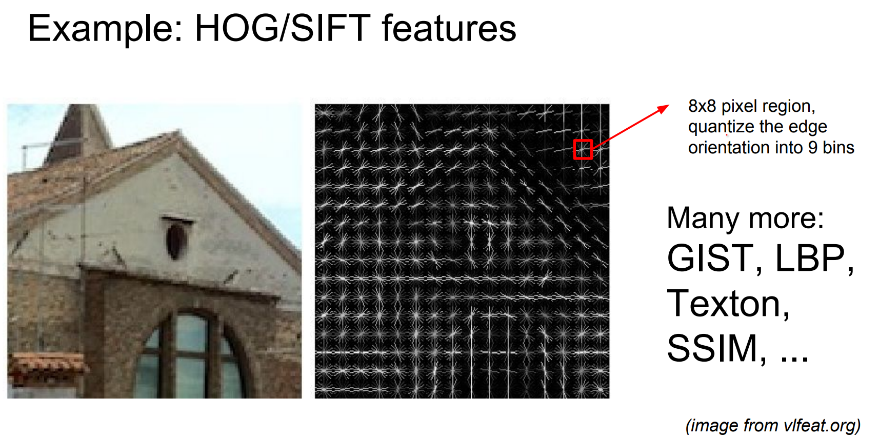
Other classics: GIST, LBP, textons, SSIM, etc.

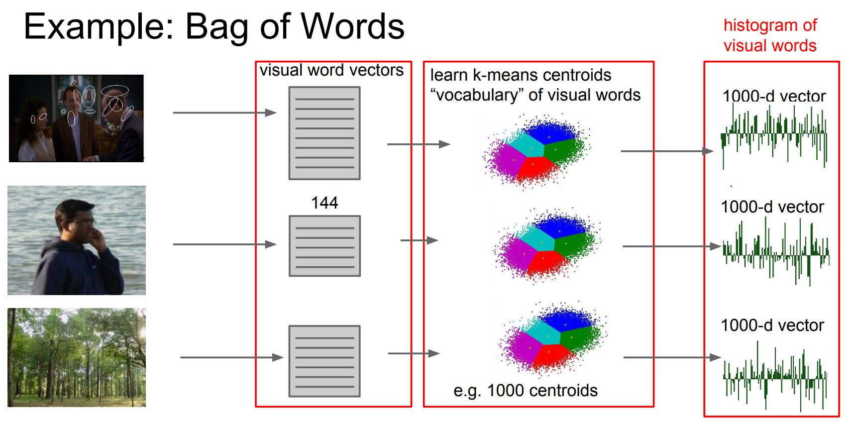
Pipeline recap:

1. Look at different image patches - parts of image.
2. Describe each patch via hand-crafted statistics (frequencies, colors, orientations).
3. Build a dictionary (cluster centers) of common patterns.
4. Represent every image as statistics over that dictionary. Third image? Lots of "green" dictionary entries.

Before vs After 2012

Pre-2012: engineer features, then train a linear classifier such as an SVM on top. Winning ImageNet entries were elaborate feature pipelines glued together with custom kernels.

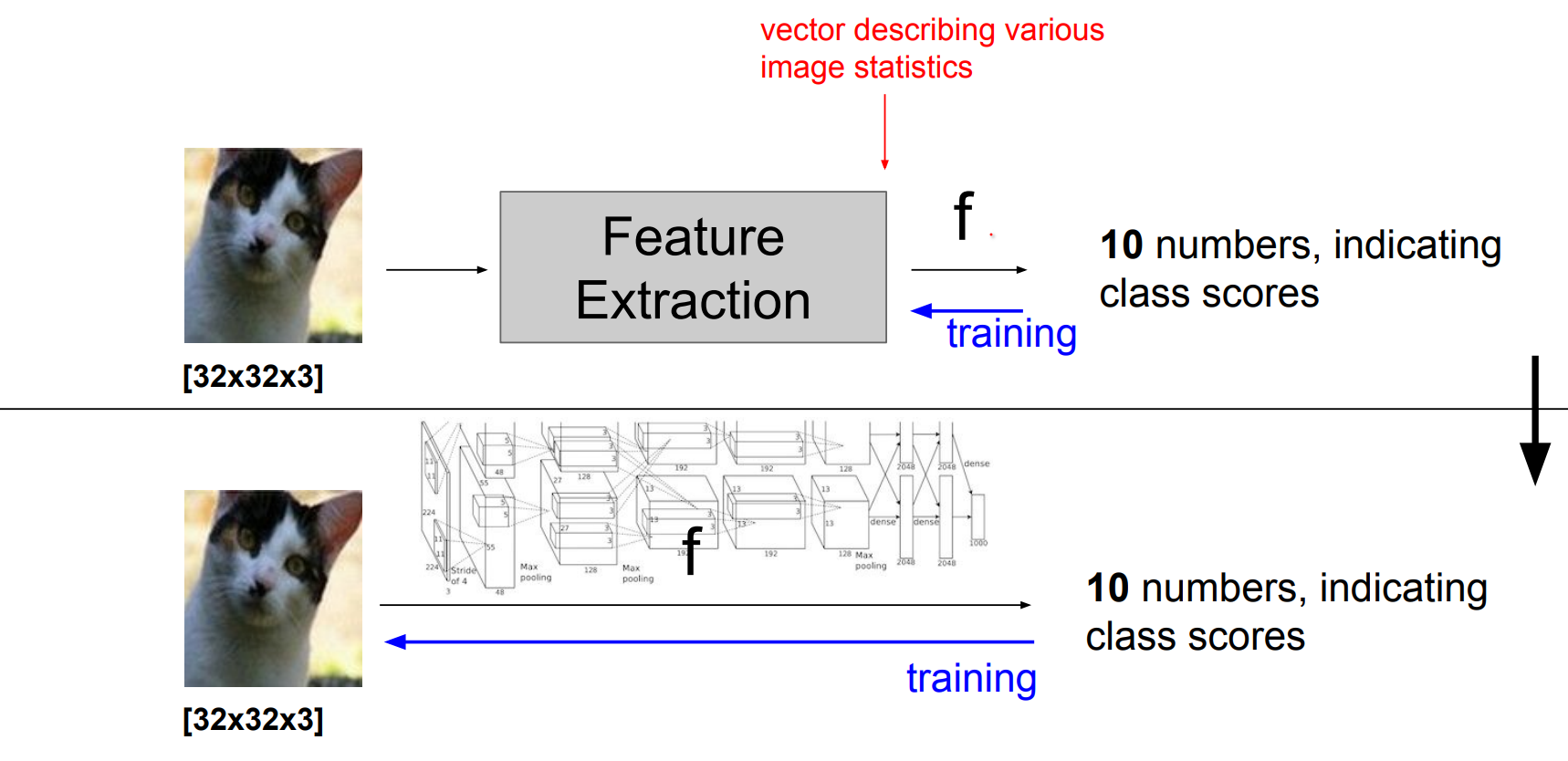
Post-2012: start from raw pixels, design neural architectures that can learn features end-to-end, and train the whole differentiable blob jointly. AlexNet’s ImageNet win nuked the feature-engineering cottage industry almost overnight.

We can train our own feature extractors. We tried to eliminate a lot of hand engineered components we want to have a single differentiable blob. So that we can train the full thing starting from the pixels.

Genius move: eliminate hand-crafted stages and let the network learn the right features directly from data. Nowadays “feature engineering” mostly means data augmentation or architecture tweaks; the network handles gradients, loss, and regularization all by itself.