5. Training Neural Networks Part 1

Part of CS231n Winter 2016

---

Lecture 5: Training Neural Networks, Part I

Here are some details about the assignments.

In this lecture, we transition from the theoretical architecture of neural networks to the practical reality of training them.

We have defined the score function and the loss function, and we know how to compute gradients via backpropagation. Now we must navigate the optimization landscape.

Project Proposals and Advice

Before beginning the technical content, a few words on course projects.

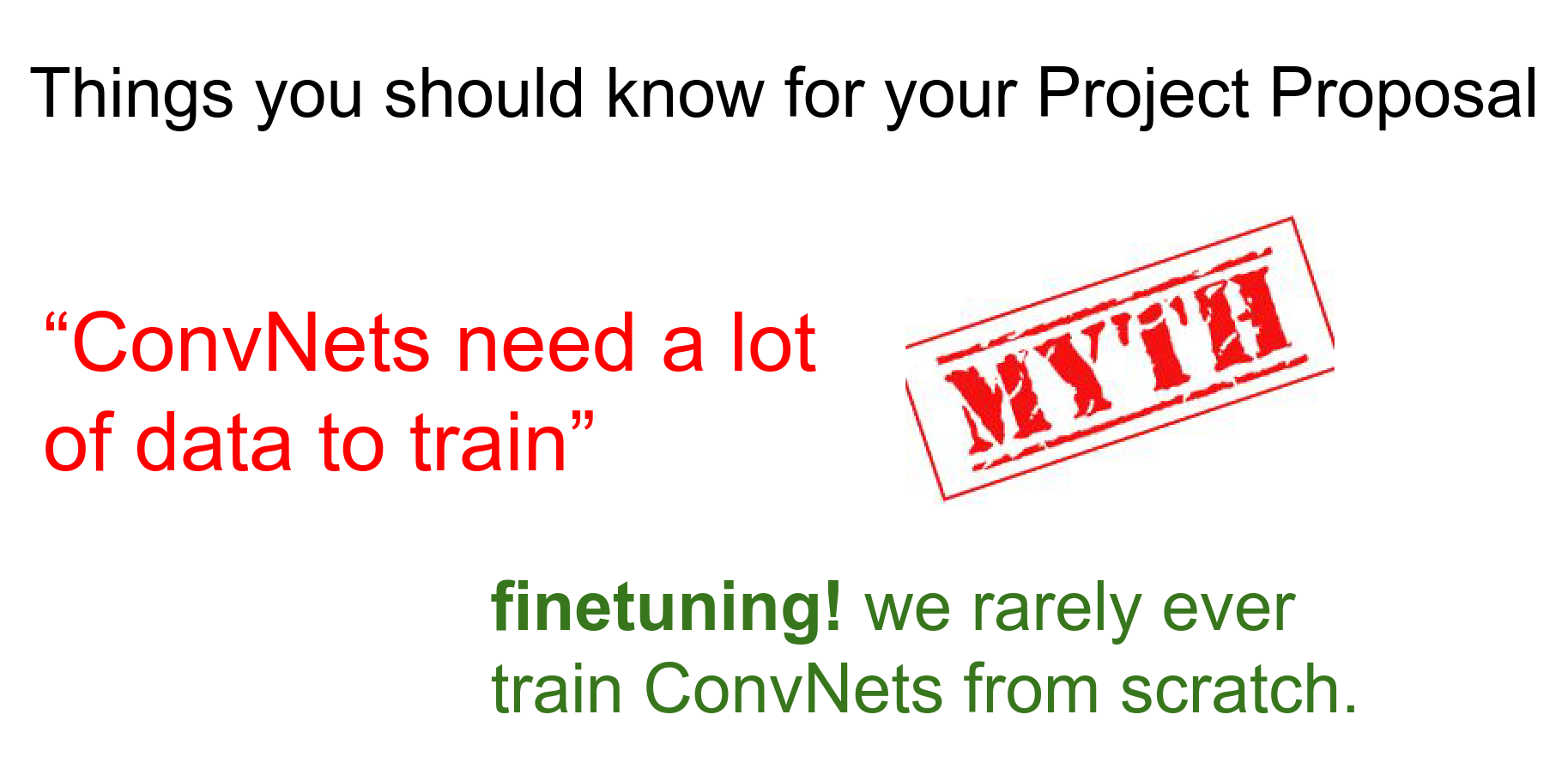
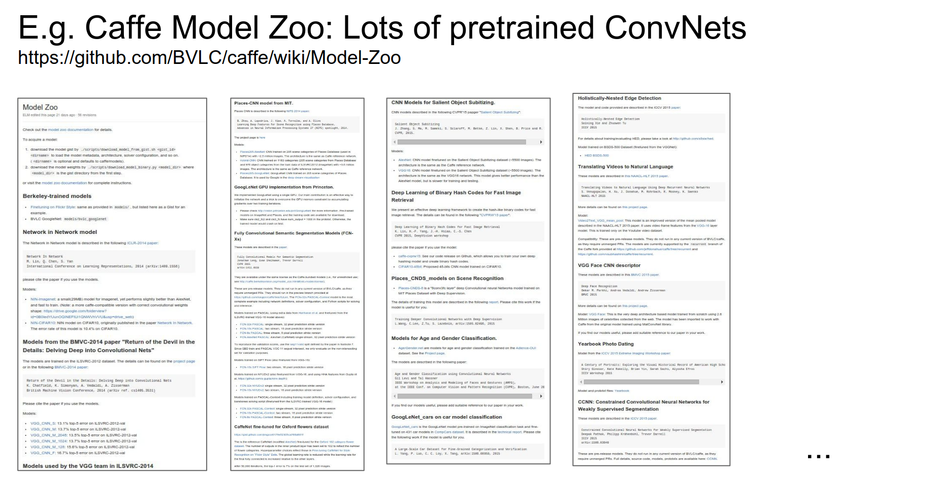
One effective strategy is fine-tuning. You rarely need to train a network from scratch. Instead, you can take a pre-trained model (trained on a large dataset like ImageNet) and adapt it to your specific problem.

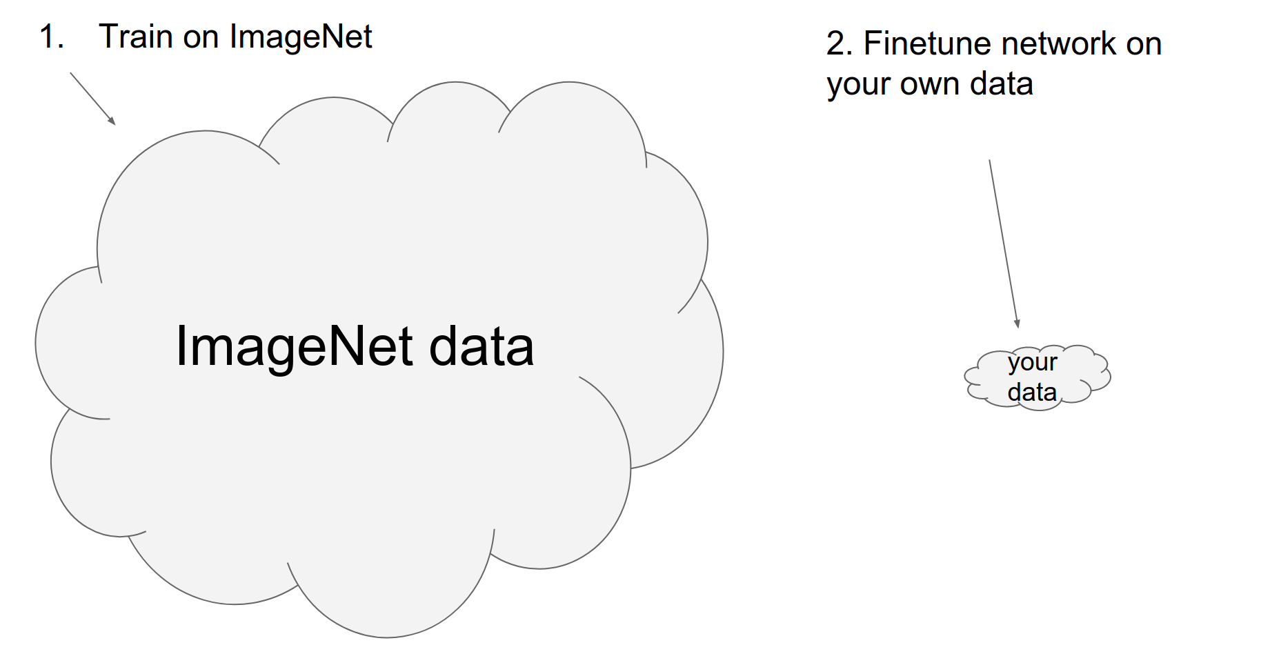
You can "chop off" the final classification layer and treat the rest of the network as a fixed feature extractor, training only a new linear classifier on top. Alternatively, you can fine-tune the entire network.

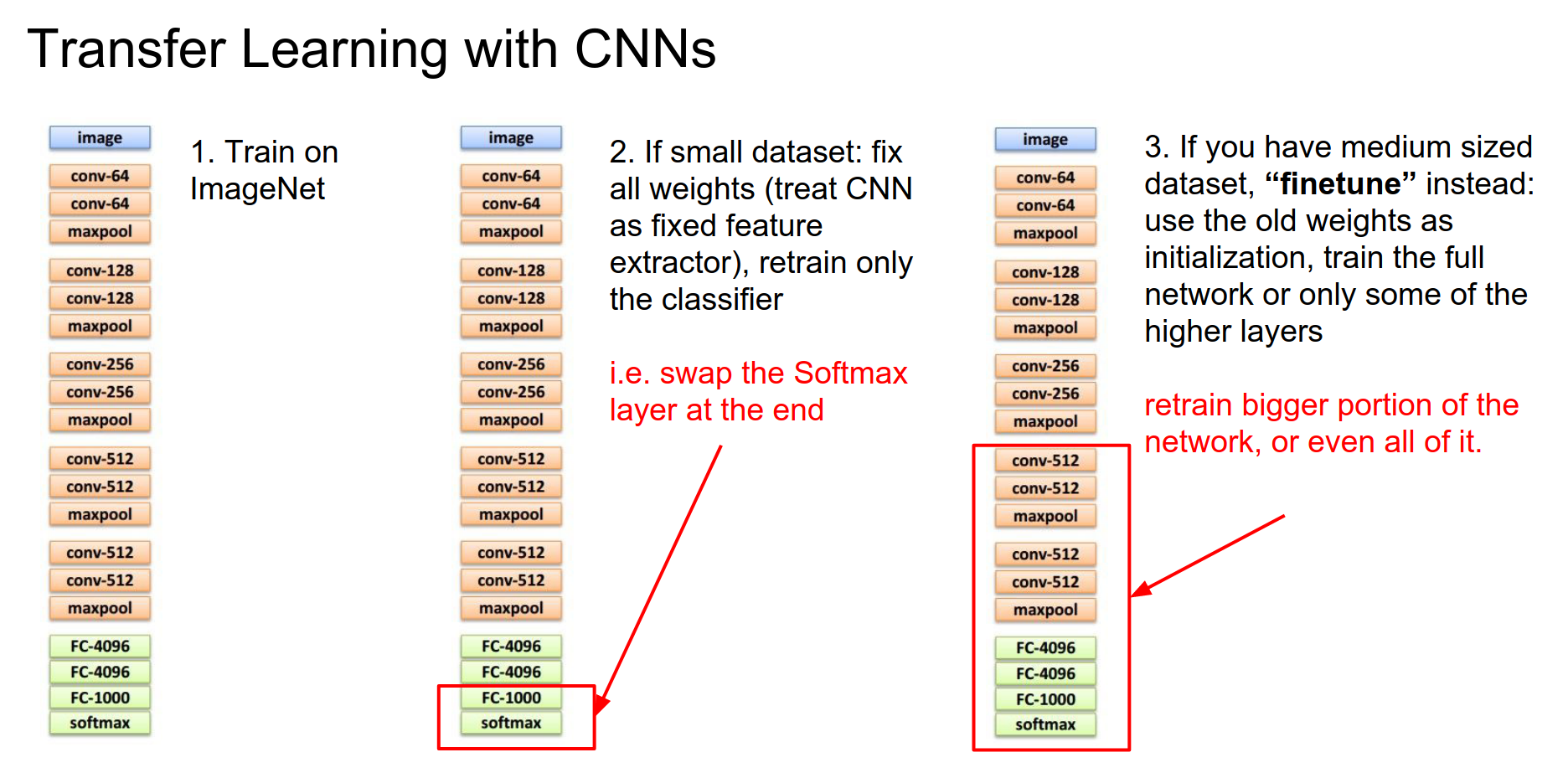
There are many pre-trained models available (Caffe Model Zoo, etc.) that you can leverage.

A word of caution regarding compute resources:

Hyperparameter optimization requires significant computational power. Be mindful of your resource usage, as compute is finite.

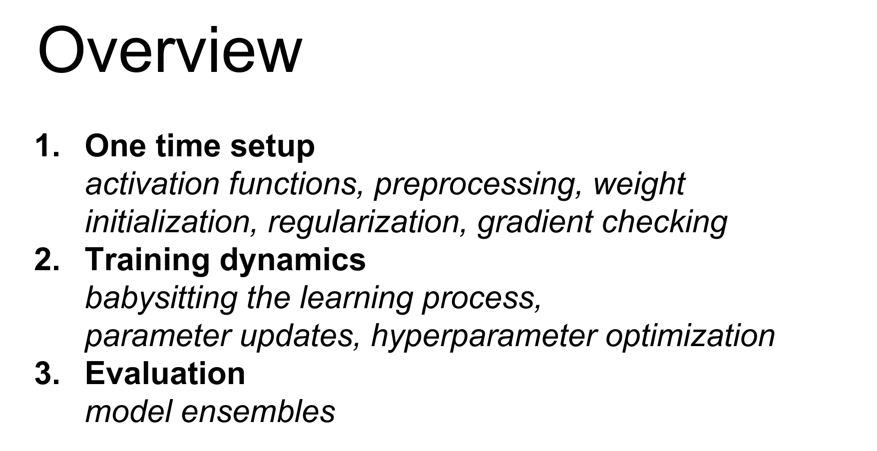
Training Overview

We are now at the stage where we loop through the training process:

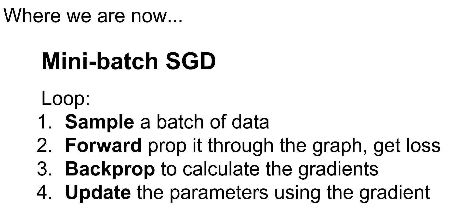
1. Sample a batch of data.
2. Forward prop to compute loss.
3. Backprop to compute gradients.
4. Update parameters.

This is an optimization problem.

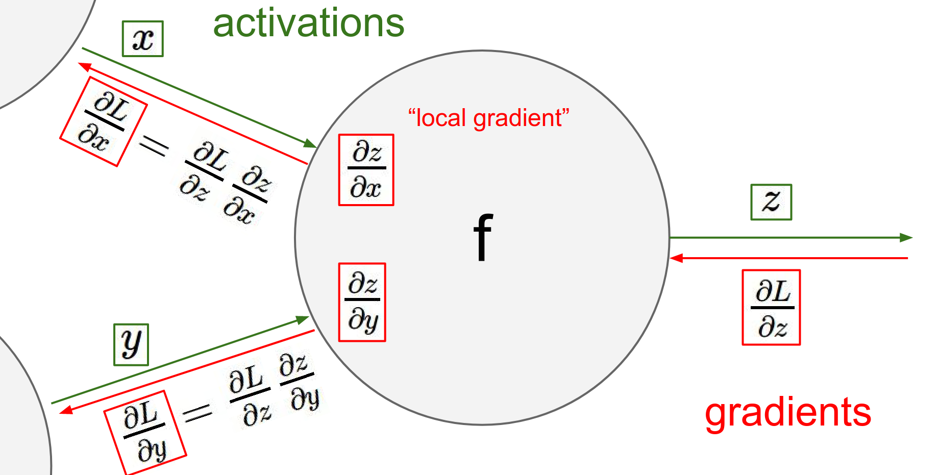
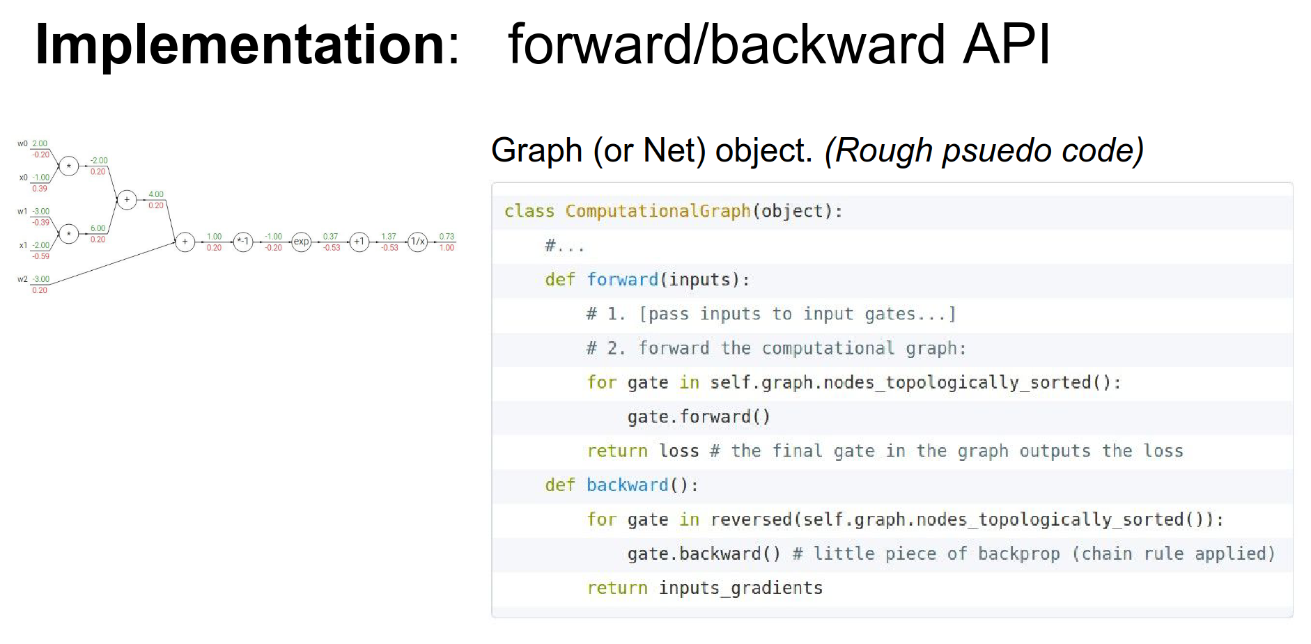
Neural networks can be incredibly large and complex.

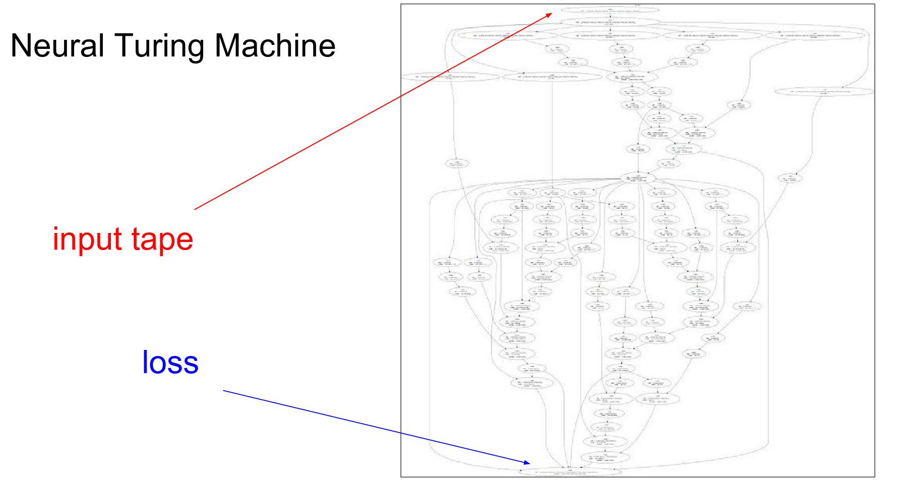
However, the complexity is managed by the chain rule. We simply need to implement the forward and backward API for each module.

For example, a simple multiplication gate:

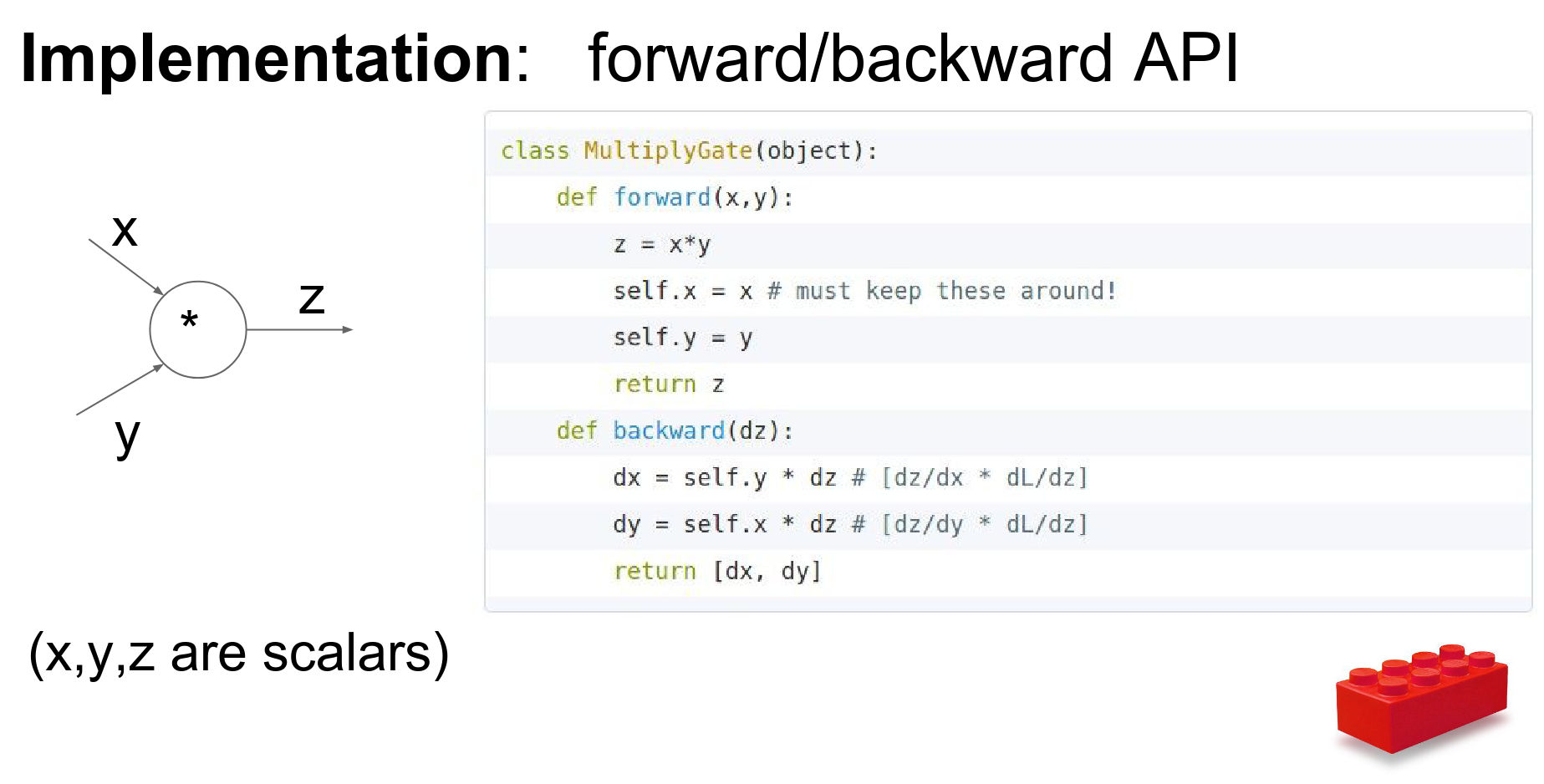
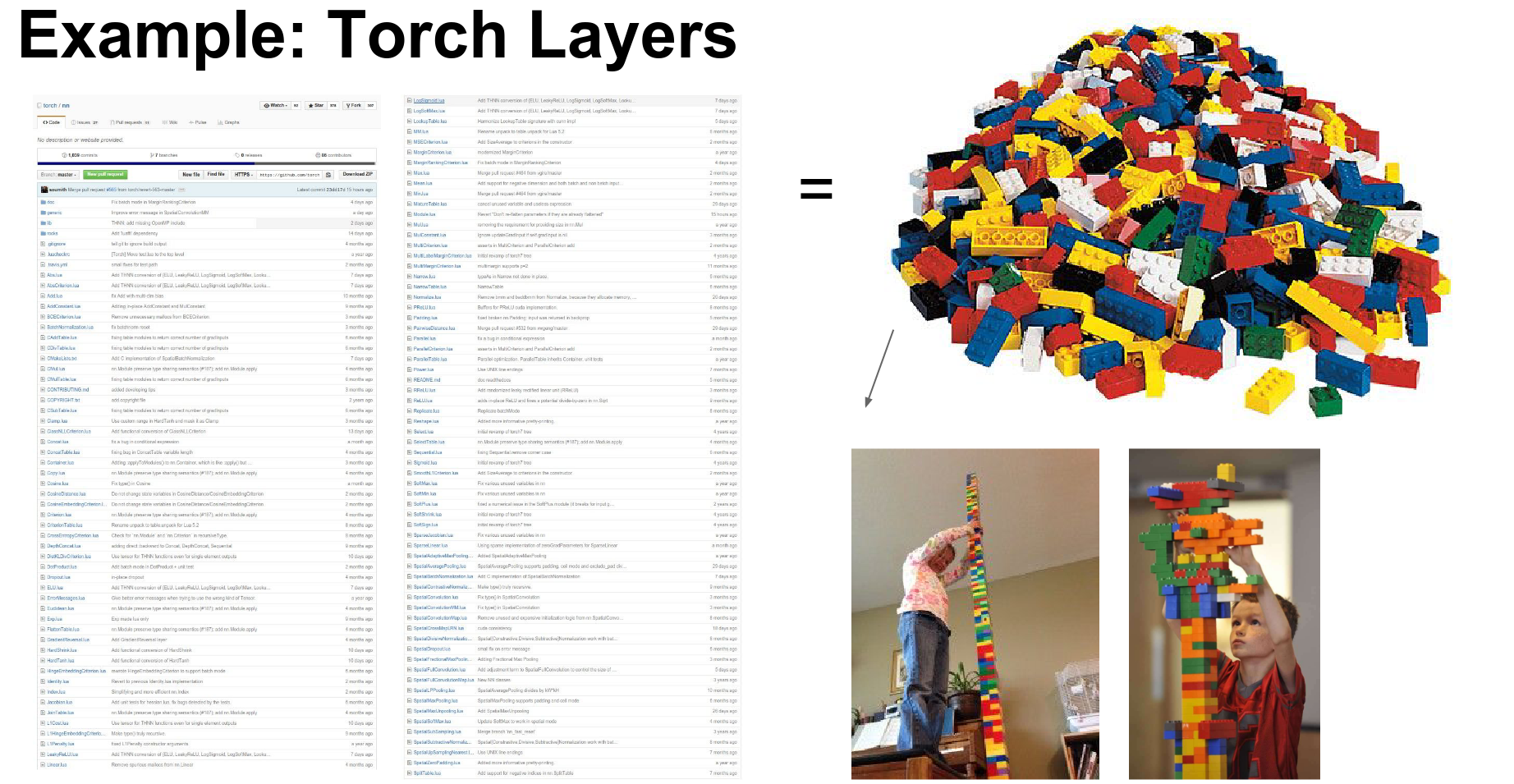
We can think of these as LEGO blocks that we stack together.

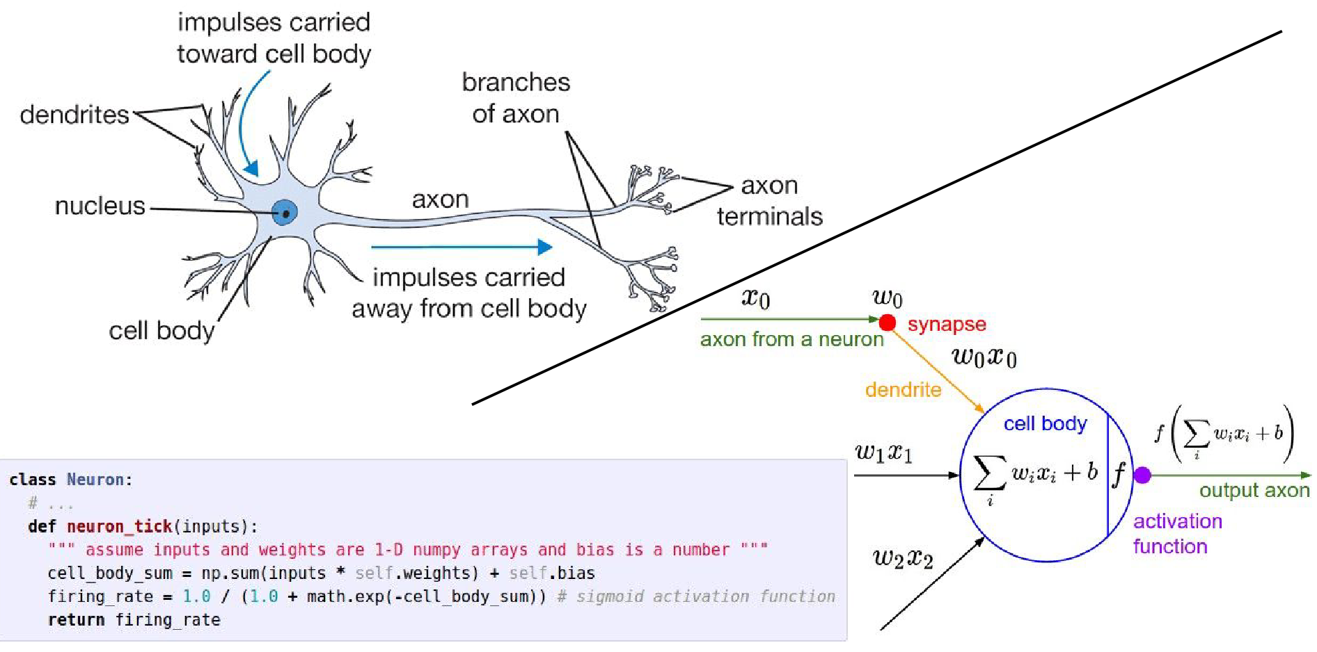
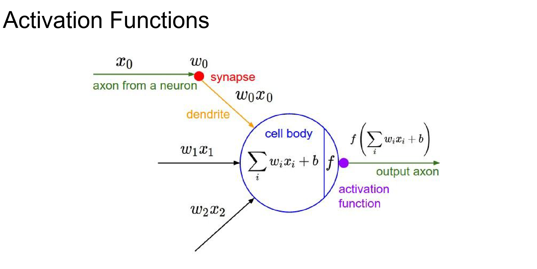
We have seen activation functions before, which introduce non-linearity.

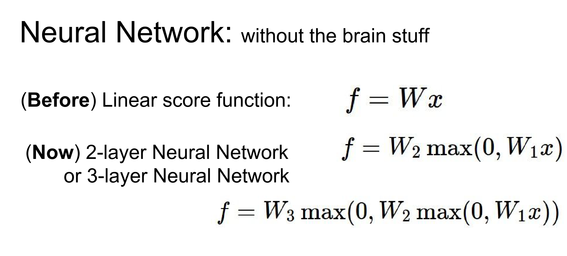
And we have discussed the loose inspiration from biological neurons.

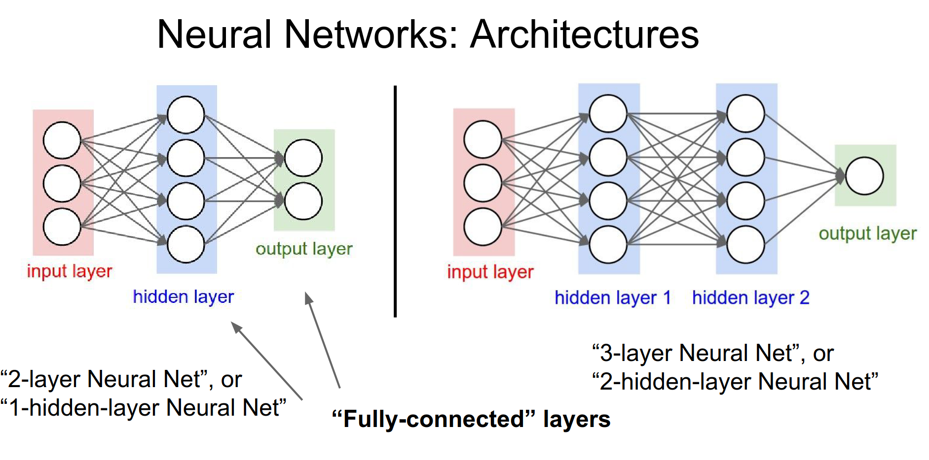
In a fully connected network, the layers with learnable weights (Fully Connected layers) are interleaved with activation functions.

History and Context

It is helpful to zoom out and look at the history of this field.

1957: The Perceptron (Rosenblatt): Early implementations were built with hardware circuits.

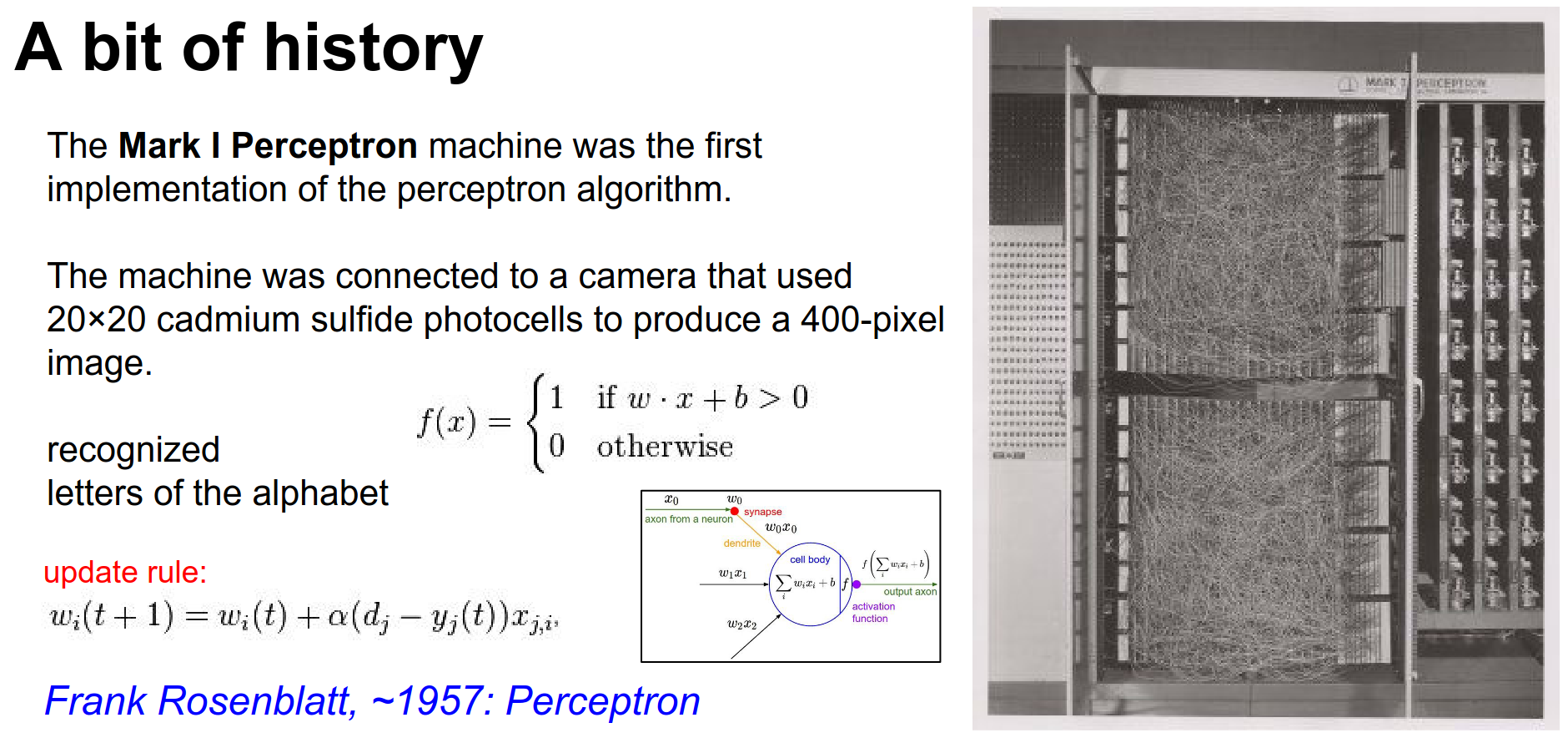
The activation function was a binary step function. Since this is not differentiable, backpropagation as we know it was not possible. They used simple update rules.

1960: Adaline/Madaline (Widrow & Hoff): Researchers started stacking these units (Multilayer Perceptron).

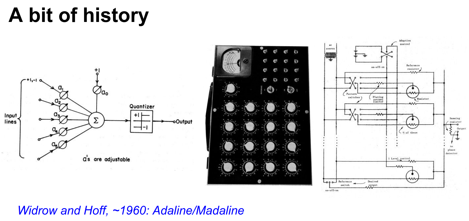
However, without a way to train the hidden layers effectively, progress stalled.

1986: Backpropagation (Rumelhart, Hinton, Williams): The field was reignited by the derivation of backpropagation, allowing training of multi-layer networks.

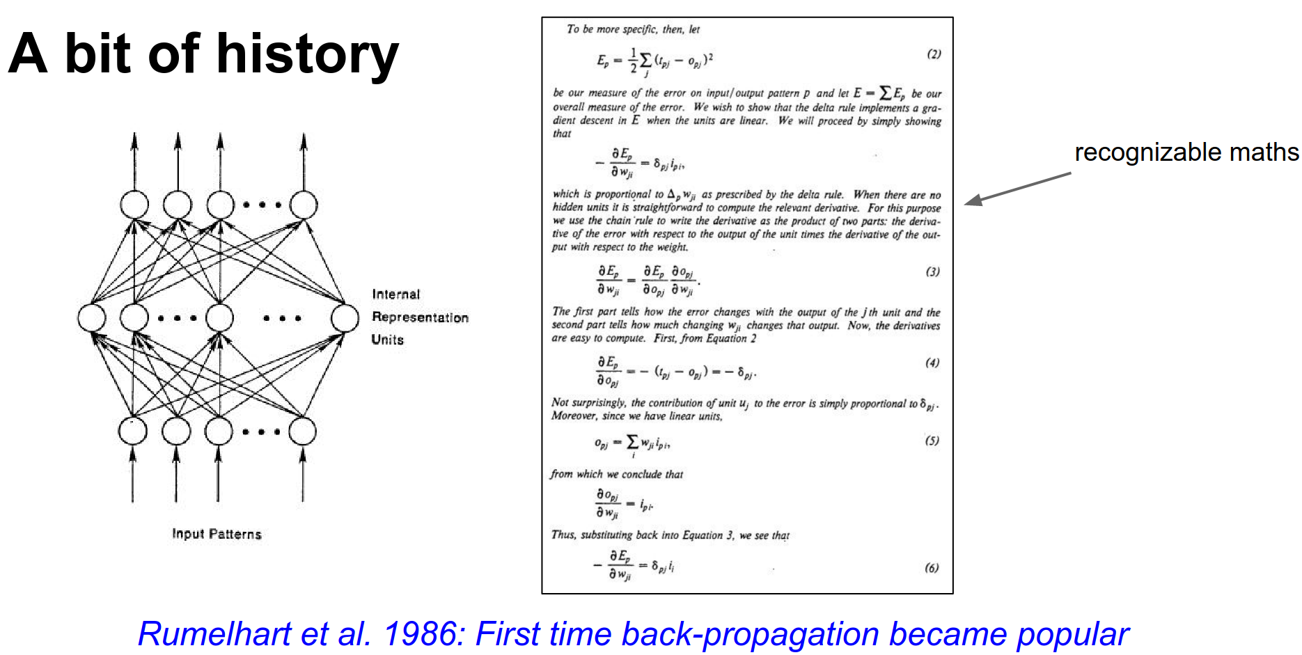
Despite the excitement, training deep networks proved difficult. Gradients would vanish or explode, and training would get stuck.

2006: Deep Learning & RBMs (Hinton, Salakhutdinov): A breakthrough came with Deep Learning. The key idea was unsupervised pre-training using Restricted Boltzmann Machines (RBMs).

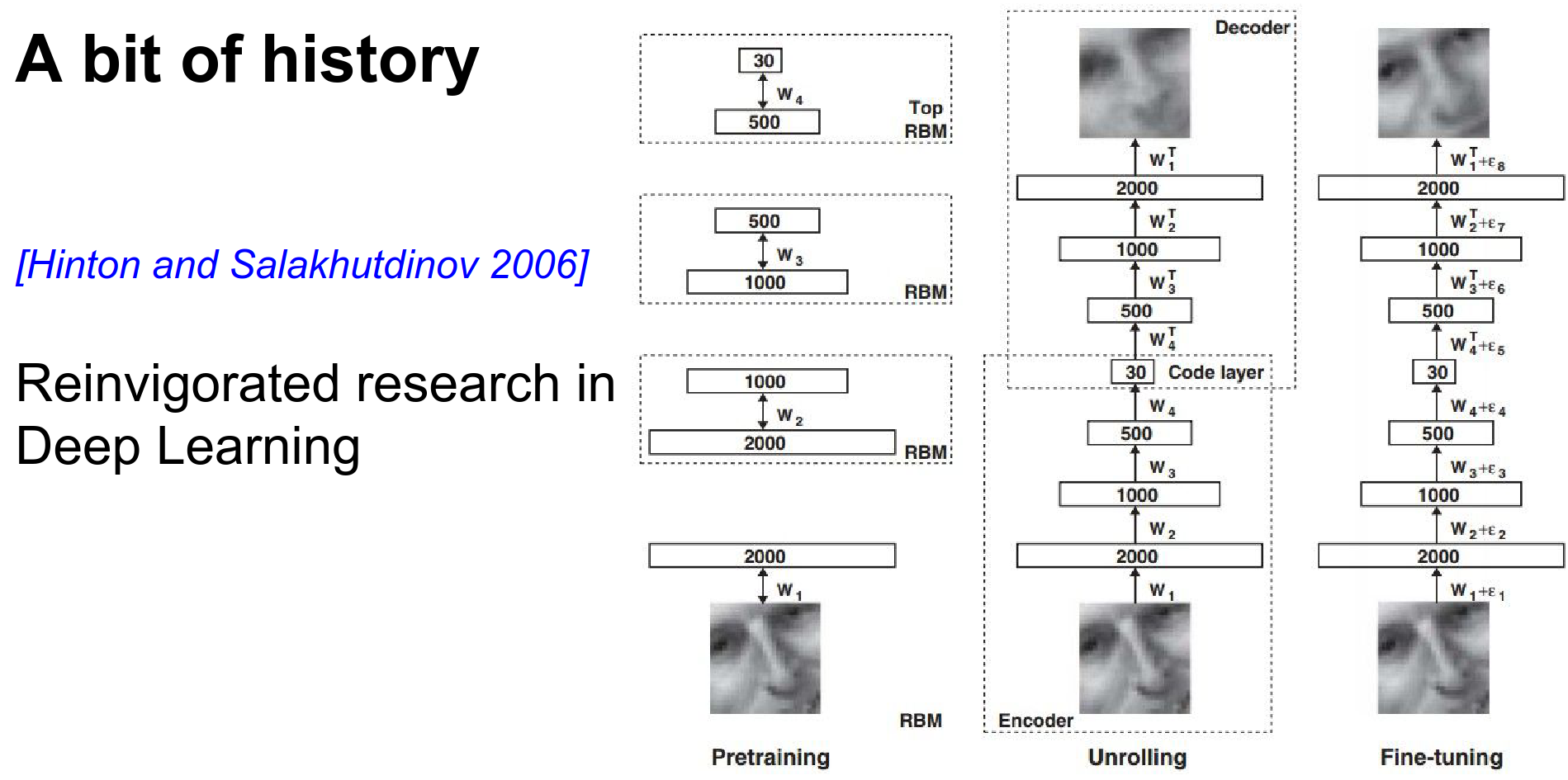
You would train the first layer to reconstruct the input, then freeze it and train the second layer, and so on. Finally, you would fine-tune the whole network with backpropagation. This initialization allowed for deeper networks.

2010-2012: The Explosion: By 2010, acoustic modeling (speech recognition) saw huge gains by replacing GMMs with Deep Neural Networks. Then came 2012.

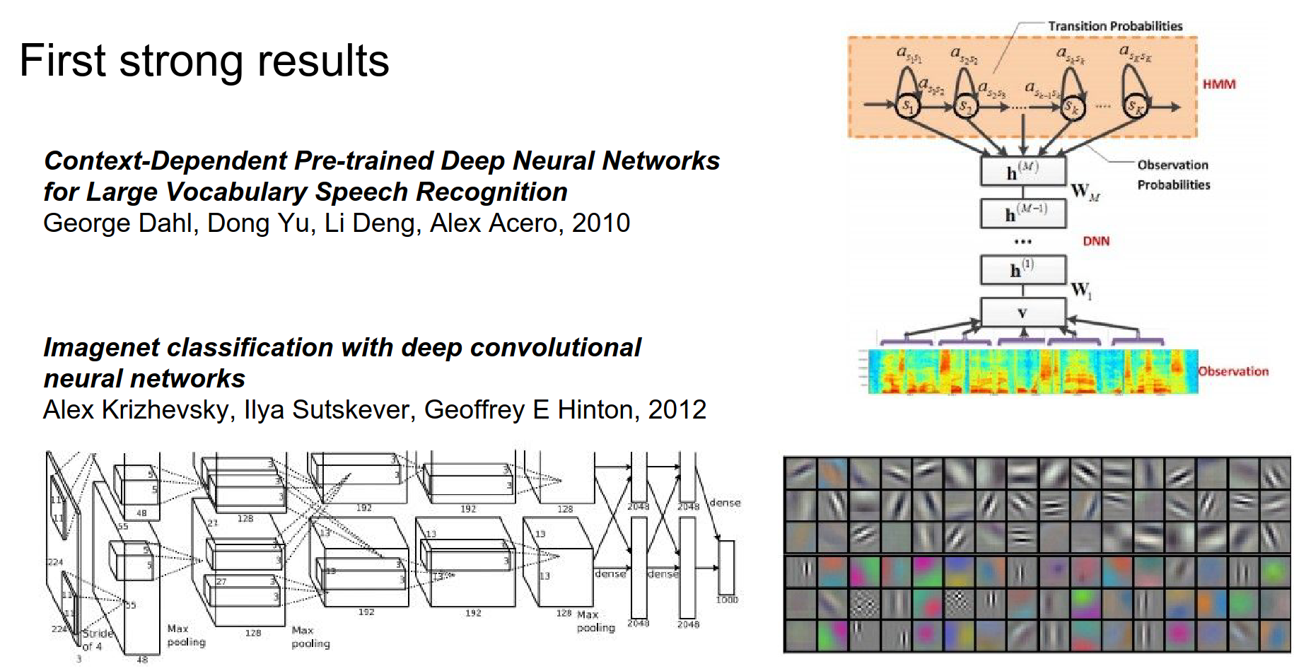
AlexNet crushed the ImageNet competition. The field exploded.

Why 2012?

• Better initialization (no longer needed complex pre-training).

• Better activation functions (ReLU).

• More data (ImageNet).

• Better compute (GPUs).

Activation Functions

We will now focus on the specific choices we make when designing and training these networks. First: Activation Functions.

There are many options available.

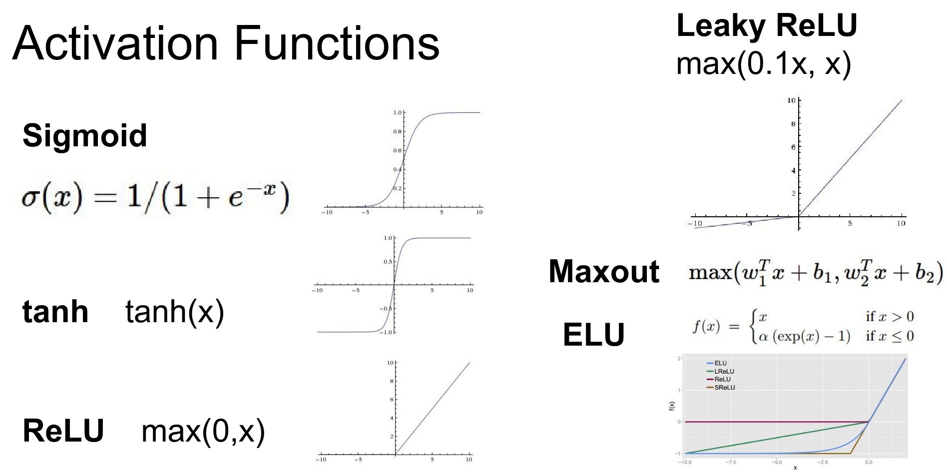
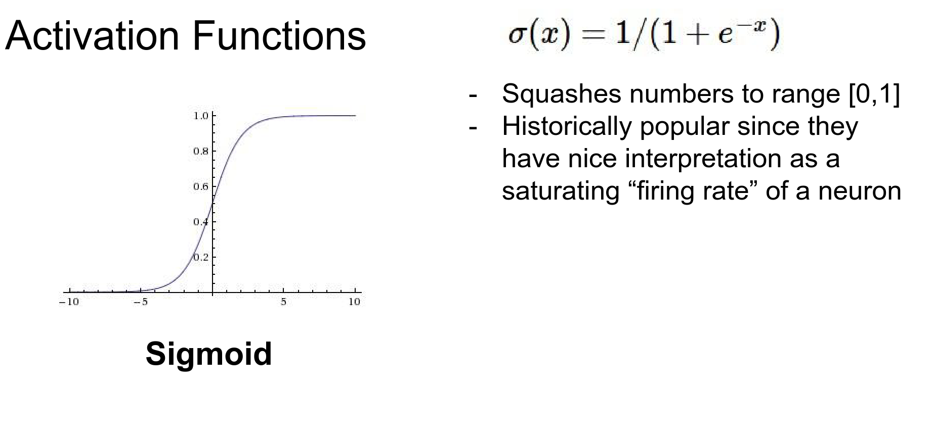
Sigmoid

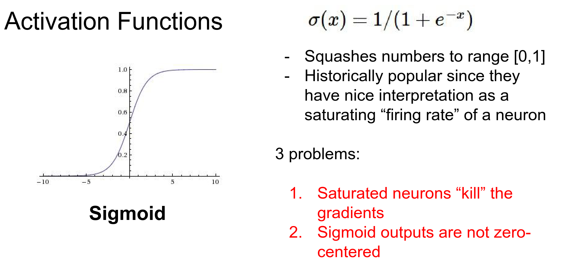
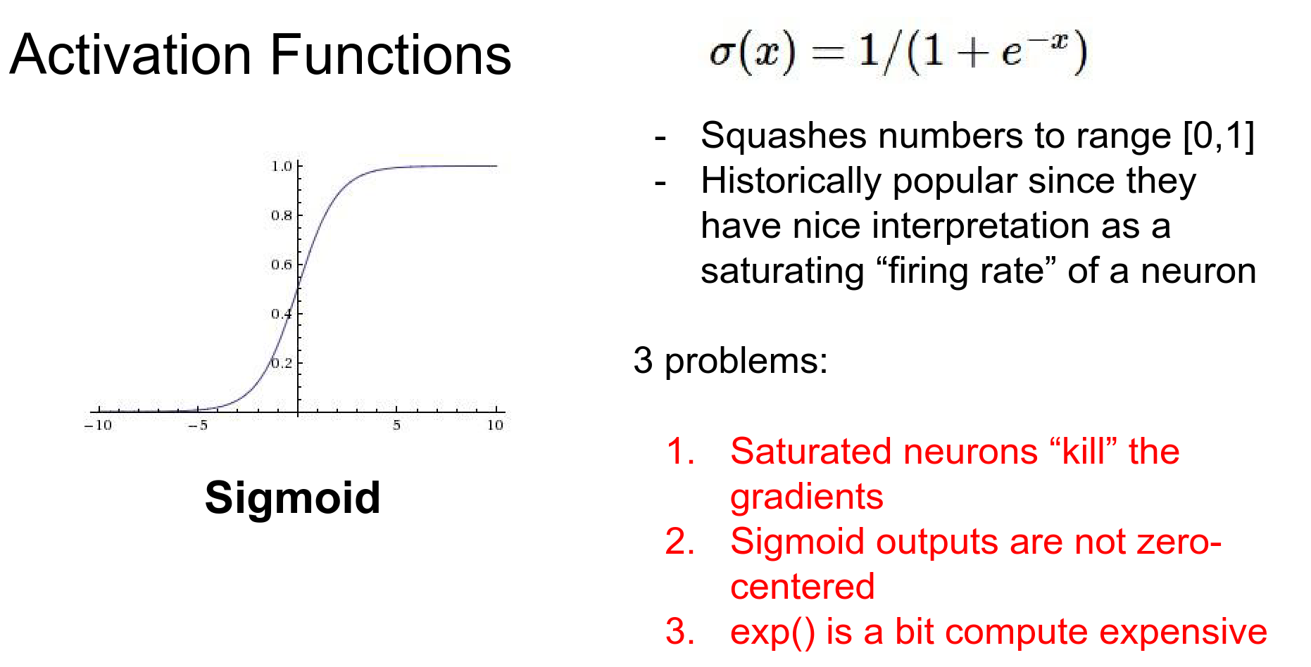
Historically, the sigmoid function was very common. It squashes real-valued inputs to the range [0, 1].

However, it has severe problems:

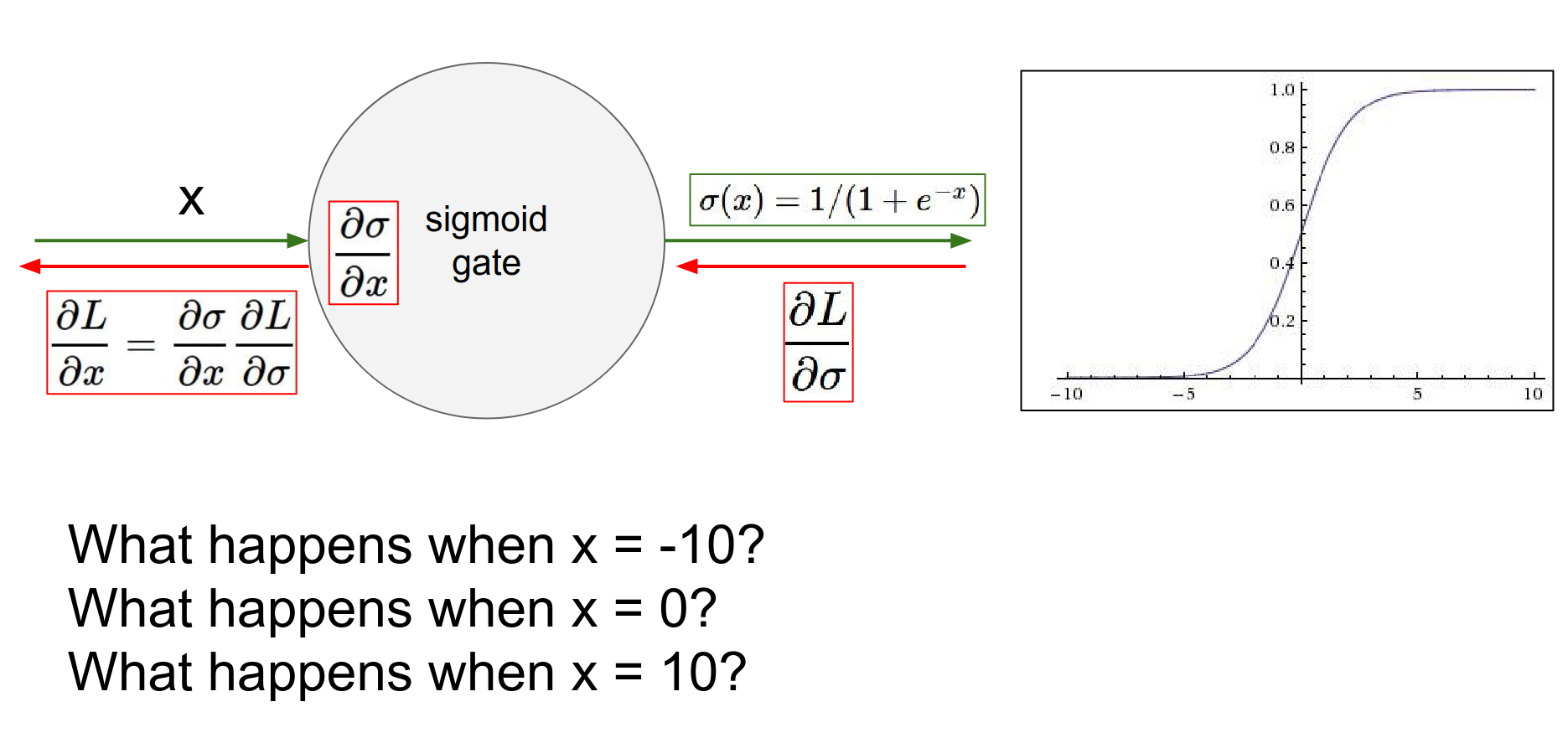
1. Vanishing Gradients: When the neuron is saturated (output close to 0 or 1), the gradient is nearly zero.

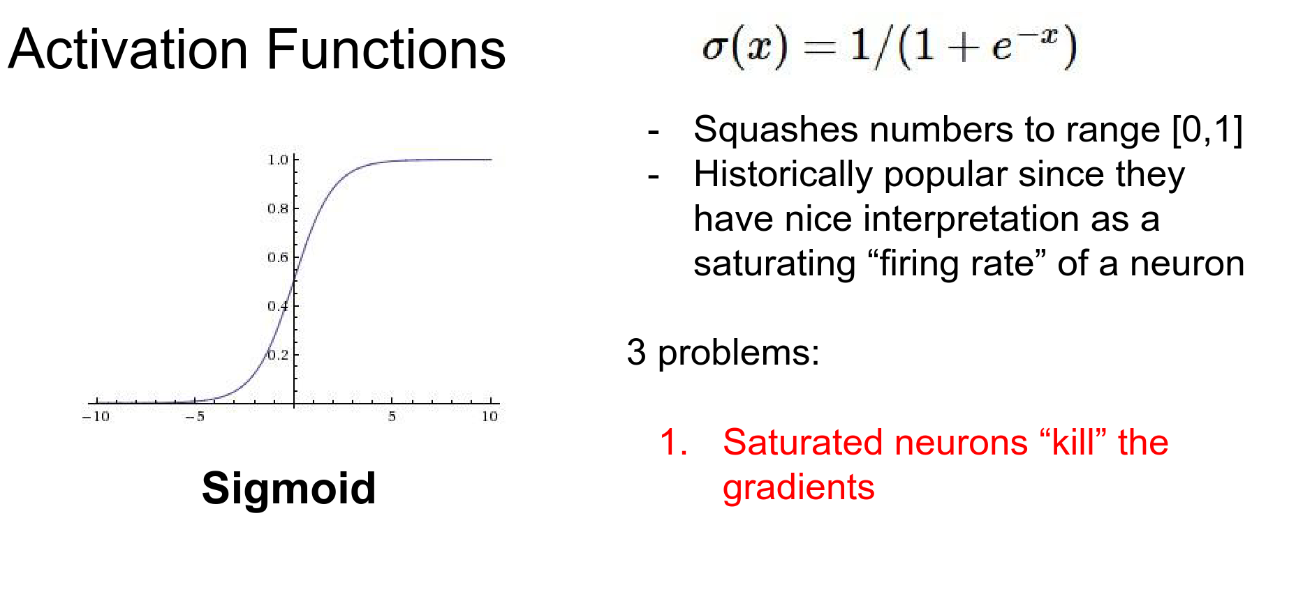
During backpropagation, this local gradient is multiplied by the upstream gradient. If the local gradient is zero, it "kills" the gradient flow to all previous layers.

1. Not Zero-Centered: The output is always positive.

If the input \(x\) to a neuron is always positive, then the gradients on the weights \(w\) will all be either positive or negative (depending on the gradient of the loss).

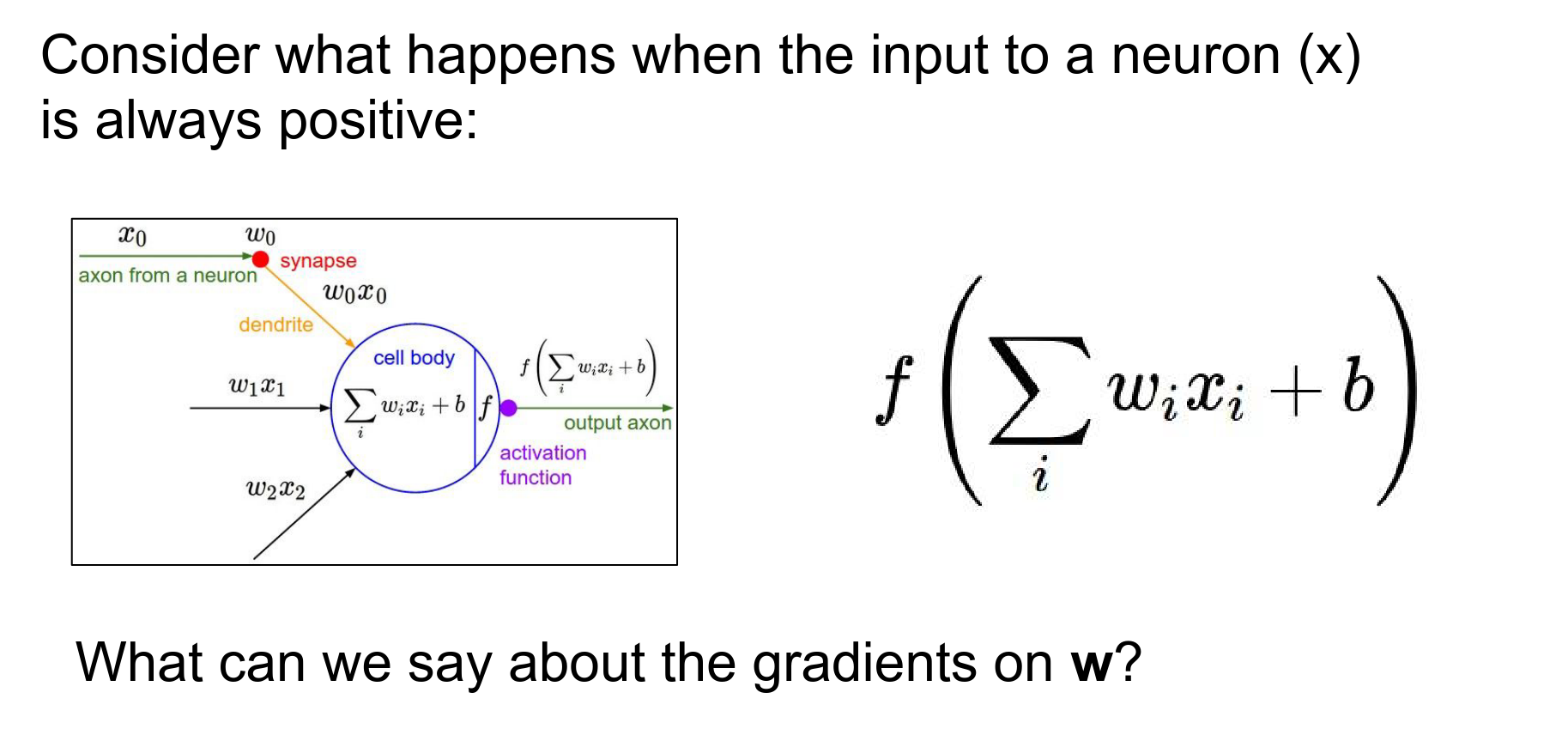
This constrains the updates to be in specific directions (zig-zagging), which is inefficient.

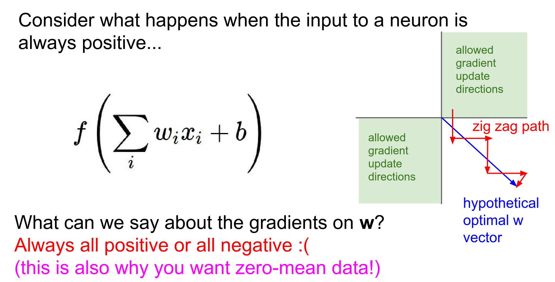
Empirically, non-zero-centered data leads to slower convergence. So you want to have things that are zero centered.

1. Expensive: The exp() function is computationally expensive compared to simple math operations.

When we are training CNN's most of compute time is actually in convolutions and dot products. So we want to make sure that we are using efficient ways to compute these.

Yann Lecun recommended using tanh() instead of sigmoids.

Tanh

The hyperbolic tangent squashes numbers to [-1, 1].

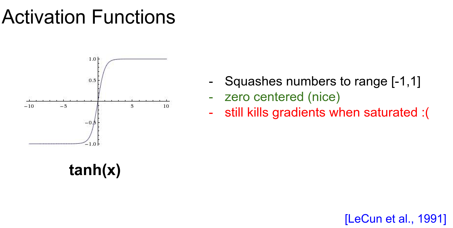
• Pros: It is zero-centered.
• Cons: It still suffers from the vanishing gradient problem when saturated.

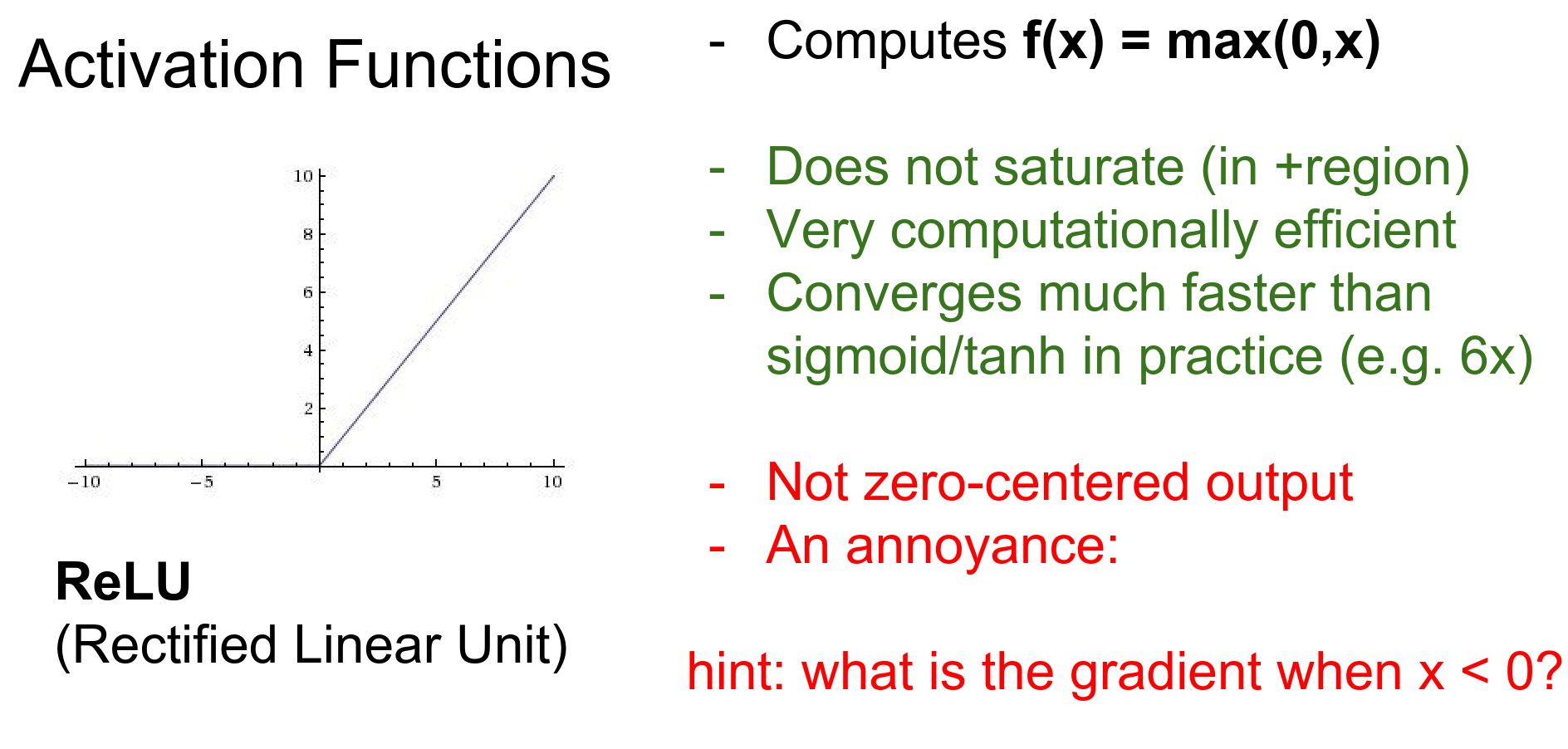
ReLU (Rectified Linear Unit)

The modern standard: \(f(x) = \max(0, x)\).

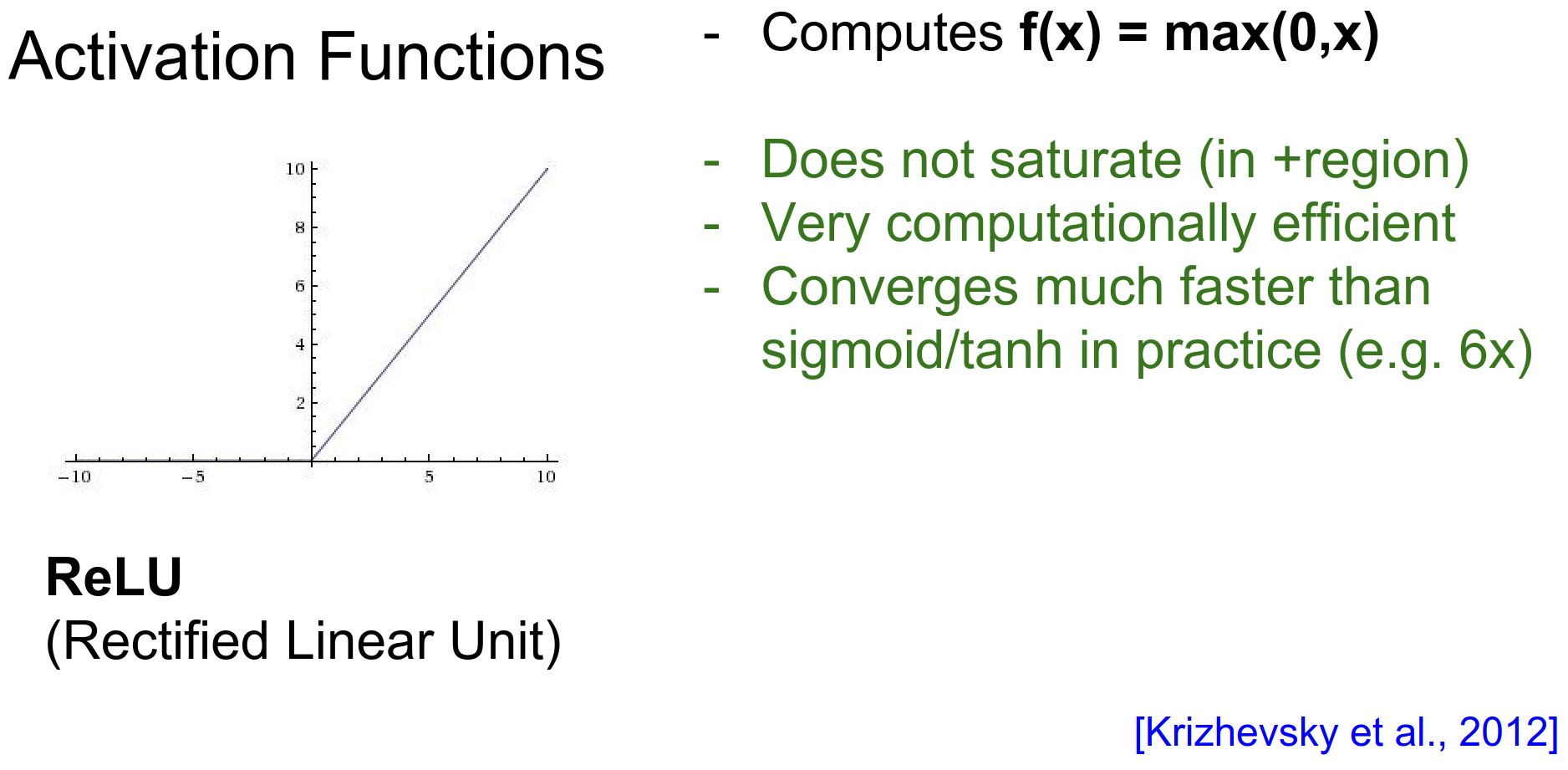
• Pros:
  • Does not saturate in the positive region.
  • Computationally very efficient.
  • Converges much faster (e.g., 6x faster for AlexNet).
• Cons:
  • Not zero-centered.
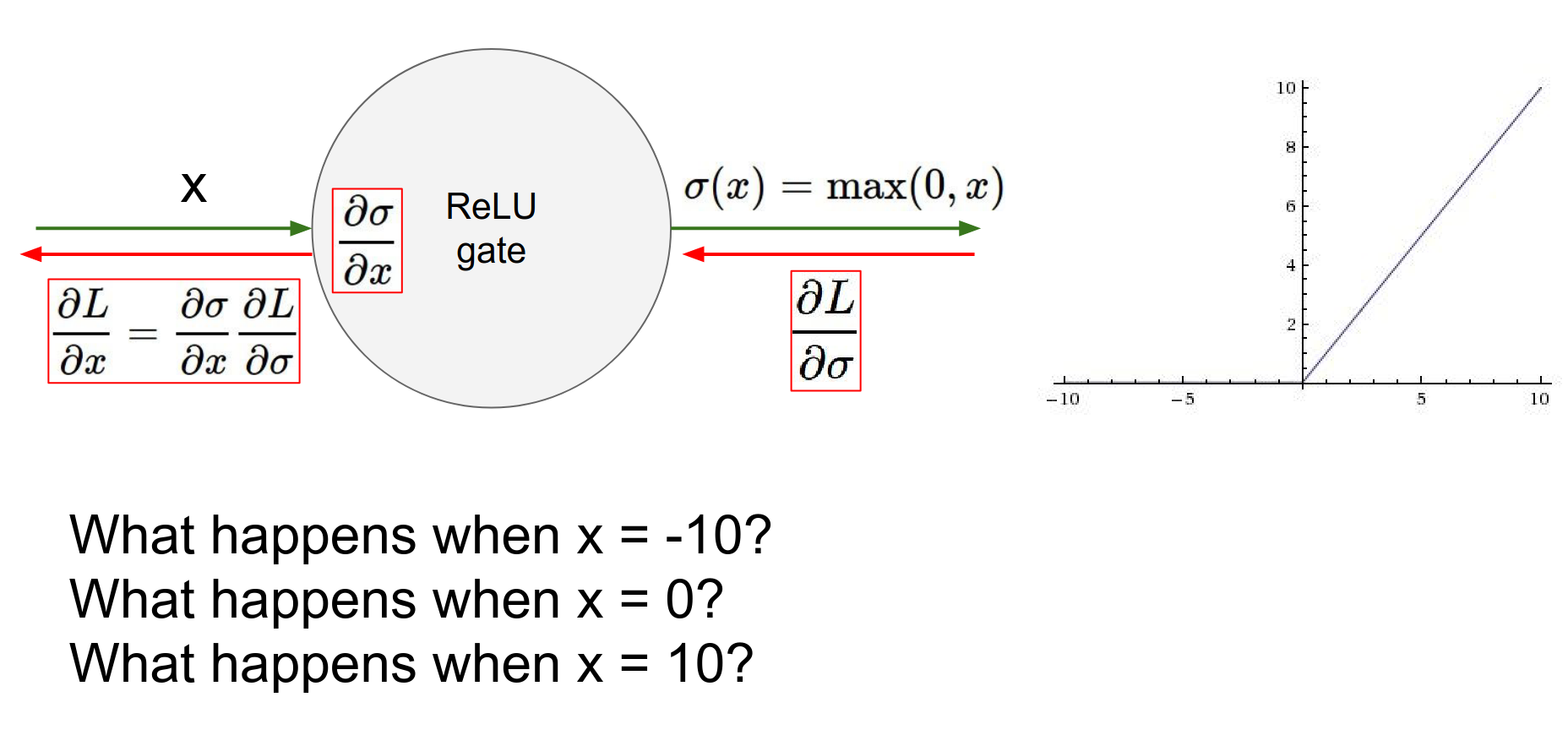
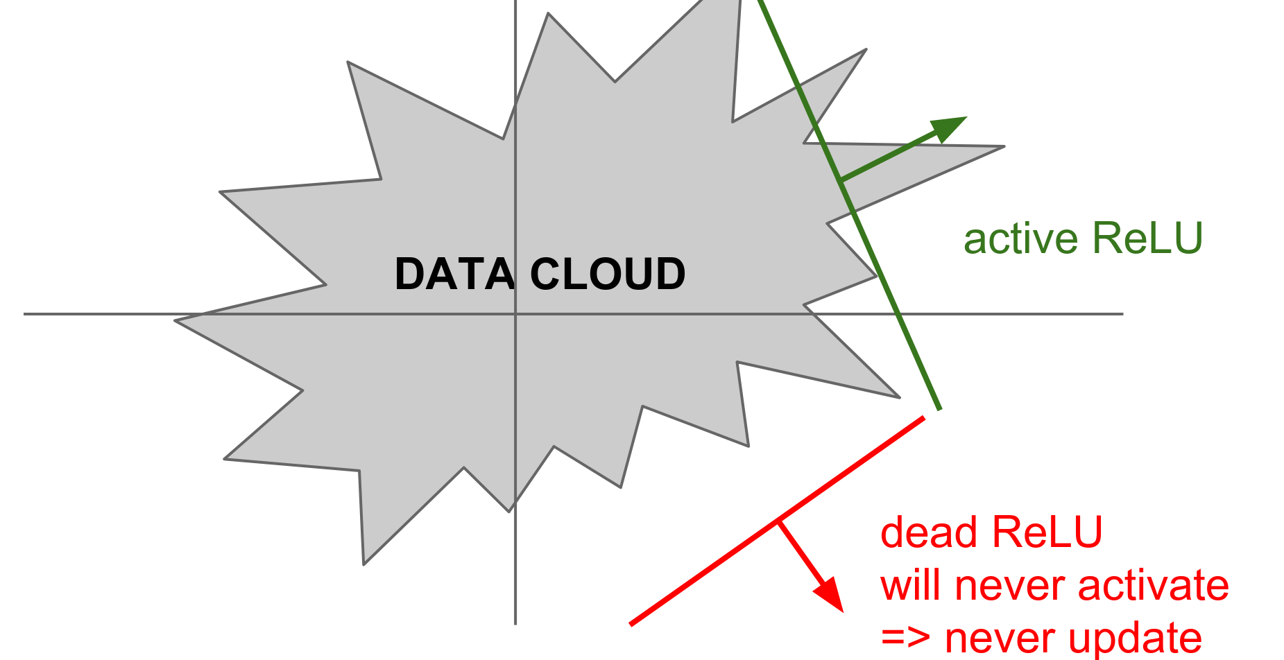
  • Dead ReLU Problem: When \(x < 0\) gradient dies.

If a neuron falls into the negative region, its output is 0 and its gradient is 0. It effectively "dies" and may never recover.

In practice, you might find that 10-20% of your network is "dead" if you are not careful.

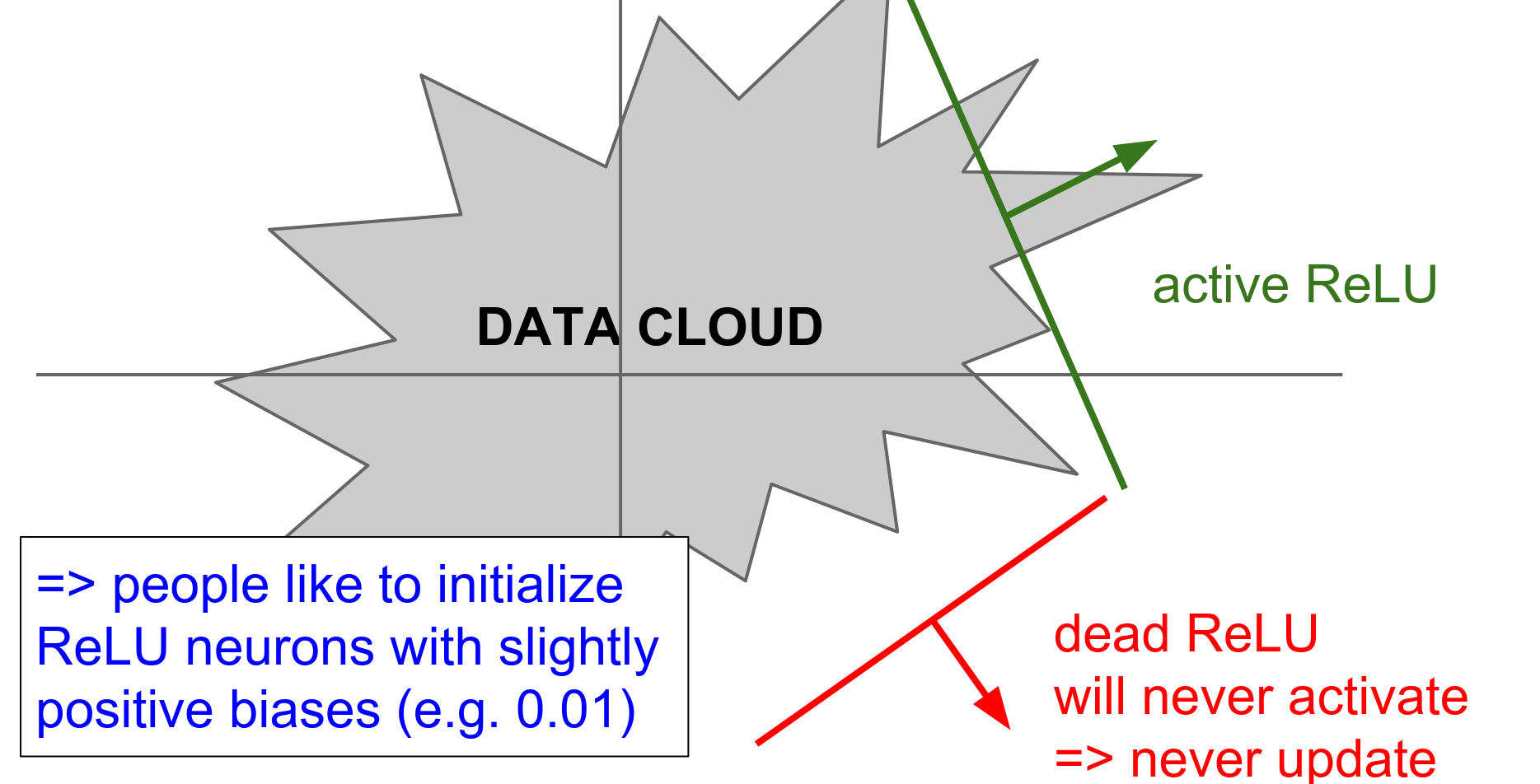
Tip: Initialize biases with a small positive number (e.g., 0.01) to ensure ReLUs start active.

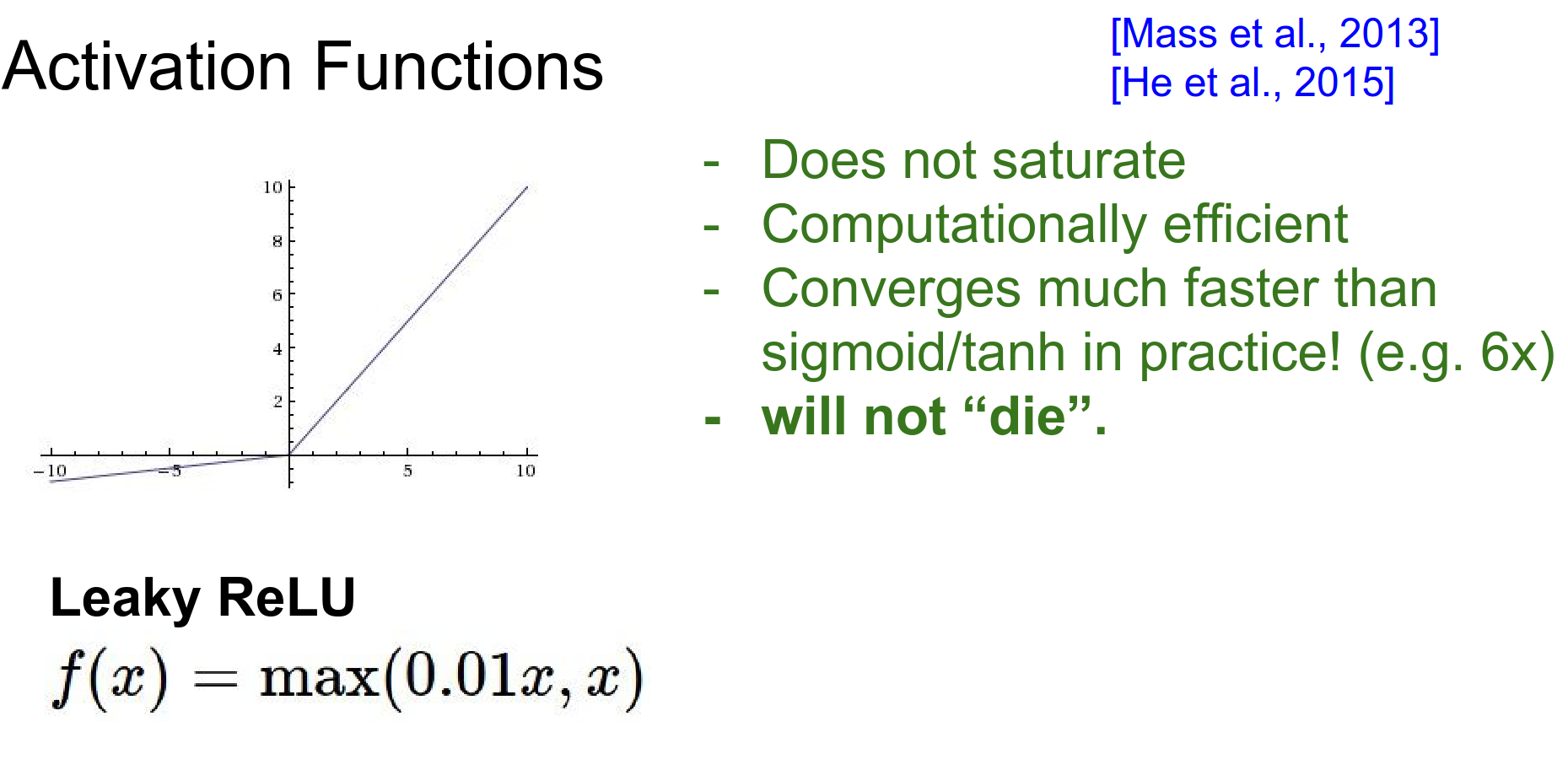
Leaky ReLU

Attempts to fix the dead ReLU problem by having a small negative slope (e.g., 0.01) when \(x < 0\).

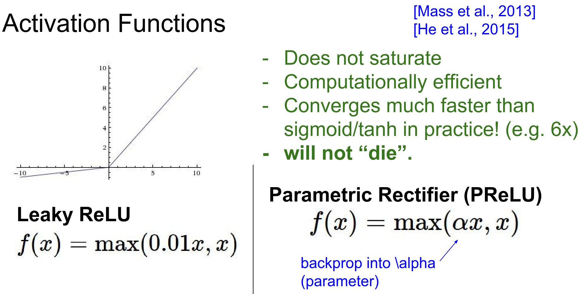
PReLU (Parametric ReLU)

The slope in the negative region is a learnable parameter \(\alpha\). Andrej is not completely sold on them.

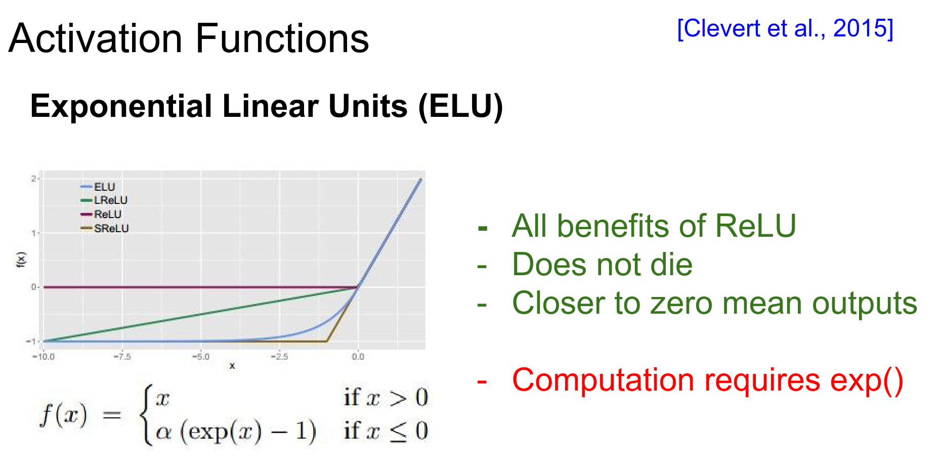
ELU (Exponential Linear Unit)

A recent proposal (Clevert et al., 2015) that has benefits of ReLU but is closer to zero mean.

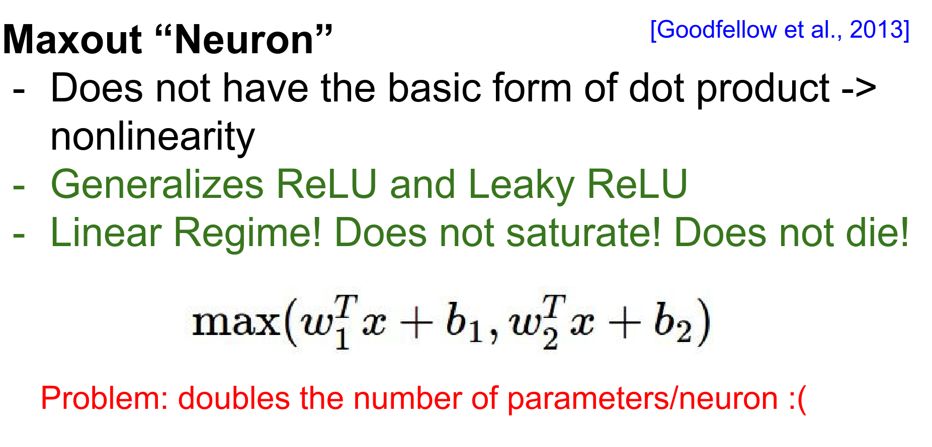
Maxout

Proposed by Ian Goodfellow et al. It generalizes ReLU and Leaky ReLU.

\(f(x) = \max(w_1^T x + b_1, w_2^T x + b_2)\)

It has no saturation and no dying ReLU problem, but it doubles the number of parameters per neuron.

Summary of Activations

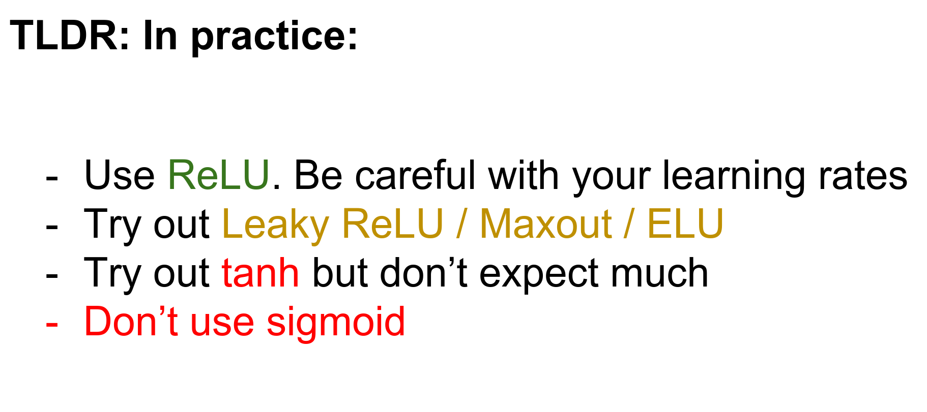
Recommendation:

• Use ReLU. Be careful with your learning rates.

• Try Leaky ReLU or Maxout.

• Try Tanh but don't expect much.

• Never use Sigmoid.

---

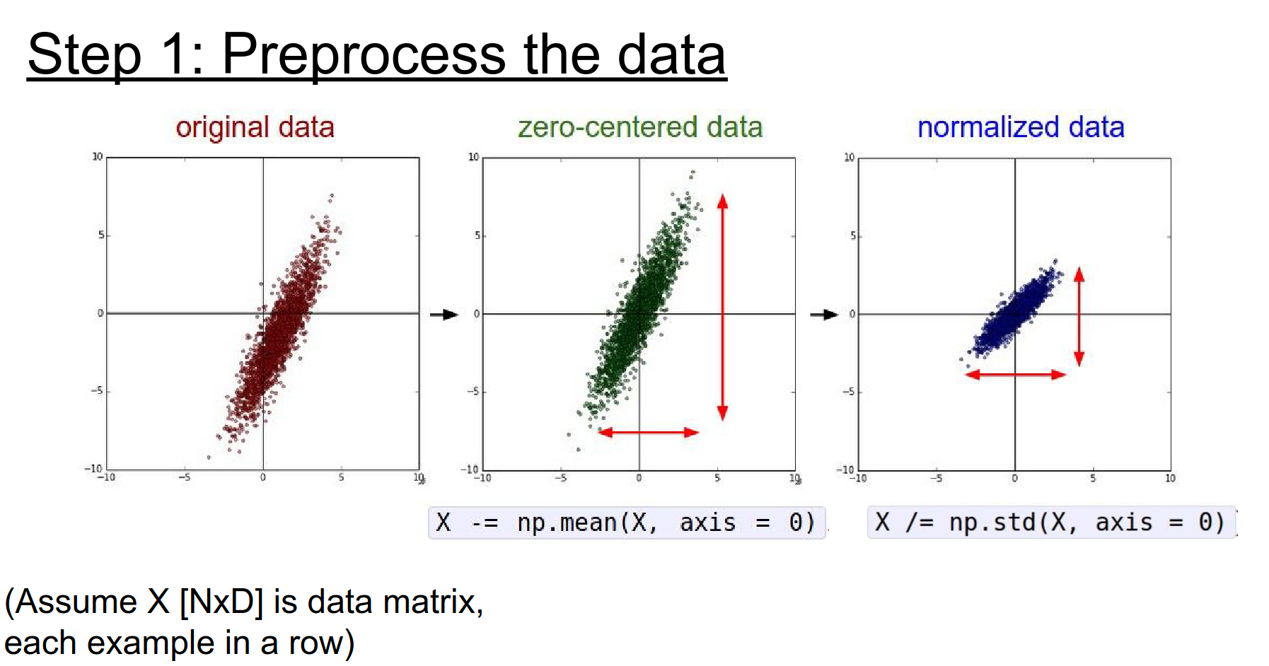
Data Preprocessing

We generally want our input data to be well-behaved.

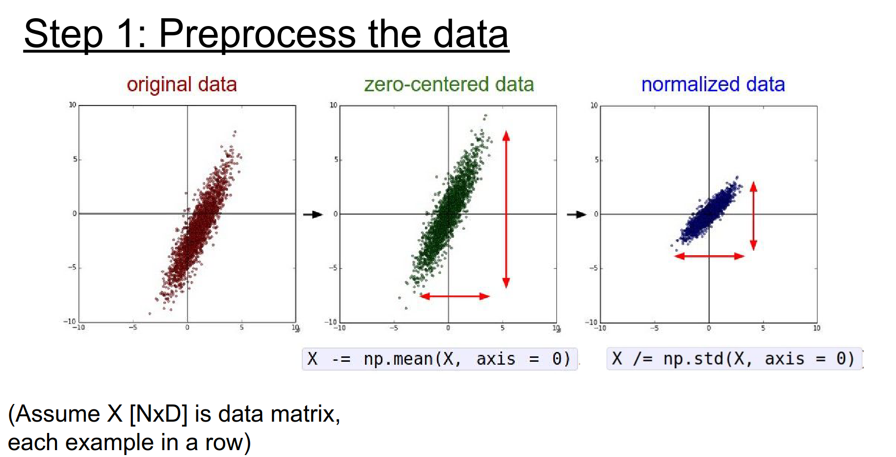
Standard practice in Machine Learning involves:

1. Mean Subtraction: Center the data around zero.

2. Normalization: Scale the data so each dimension has unit variance.

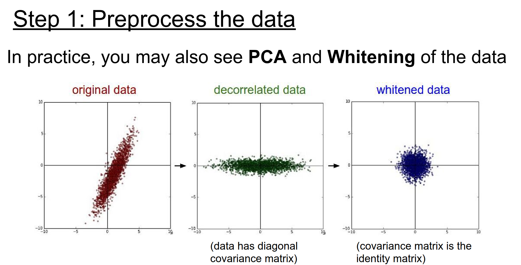
Other techniques like PCA and Whitening (decorrelating the data) are common in general ML but less common in image processing due to the high dimensionality.

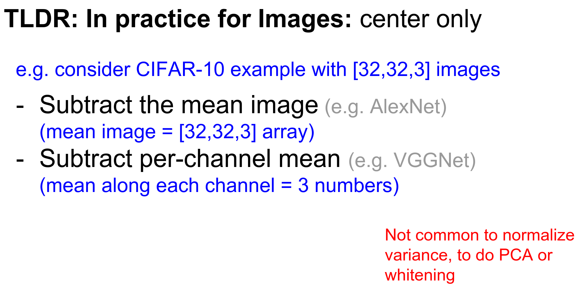
For Images:

• Subtract the mean image (e.g., AlexNet).

• Or subtract the per-channel mean (e.g., VGGNet).

• Normalization is usually not strictly necessary because pixel values are already on the same scale (0-255).

Weight Initialization

How do we start the optimization? We cannot initialize all weights to zero.

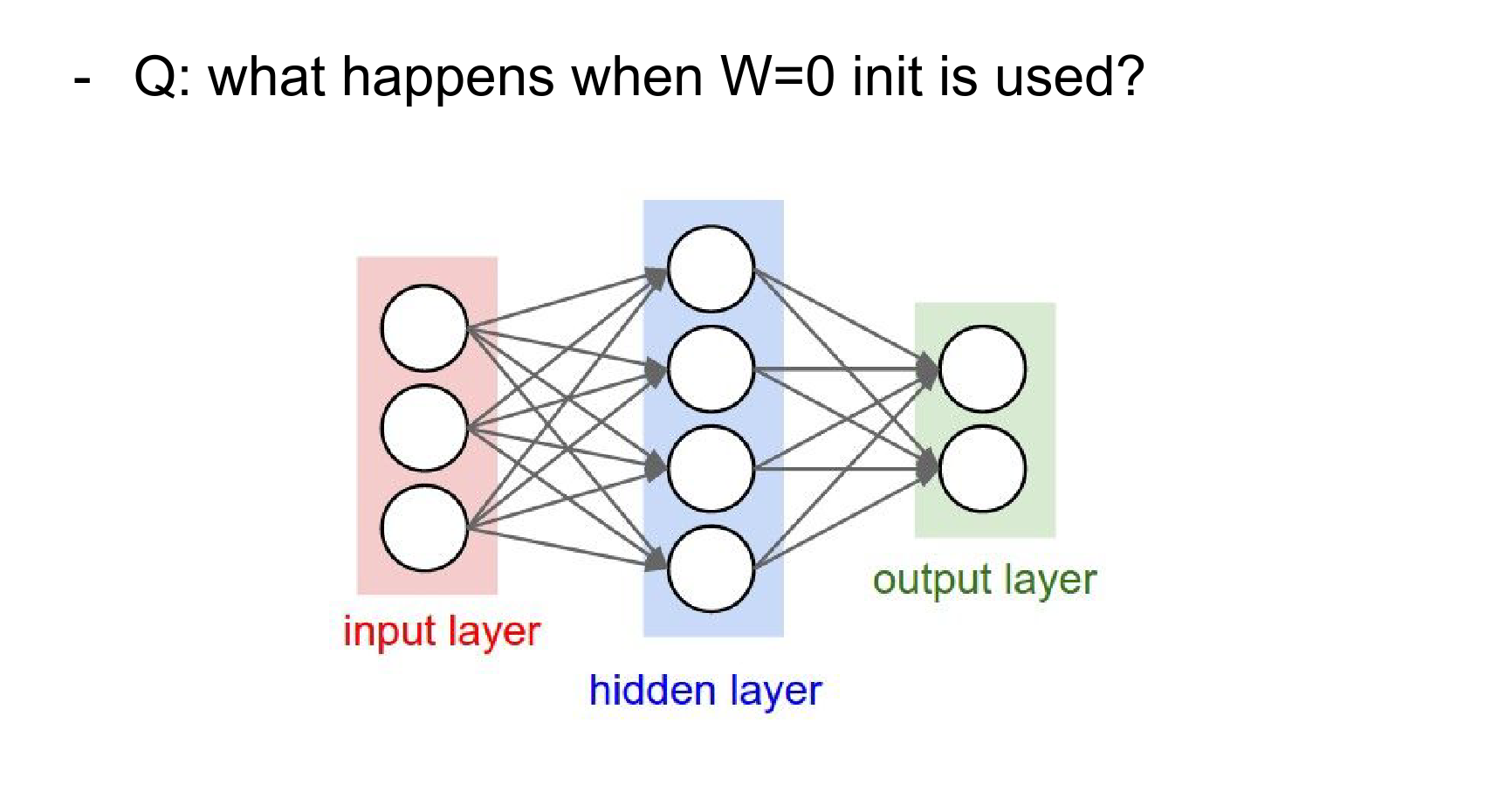
If all weights are zero, every neuron computes the same output and gets the same gradient update. There is no symmetry breaking.

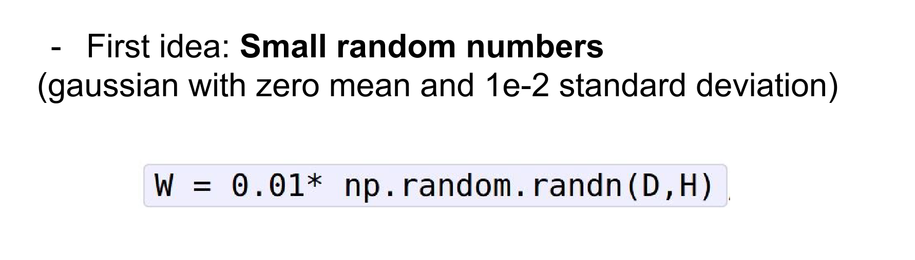
Small Random Numbers

A common first attempt is small random noise: W = 0.01 * np.random.randn(D, H).

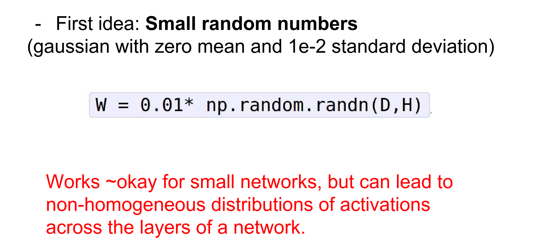
This works for shallow networks, but fails for deep ones.

Let's look at an experiment with a 10-layer network using Tanh non-linearities.

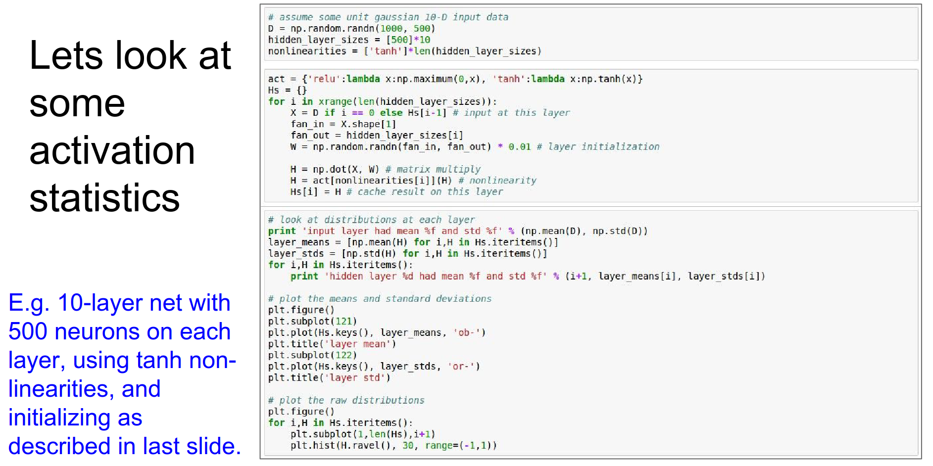
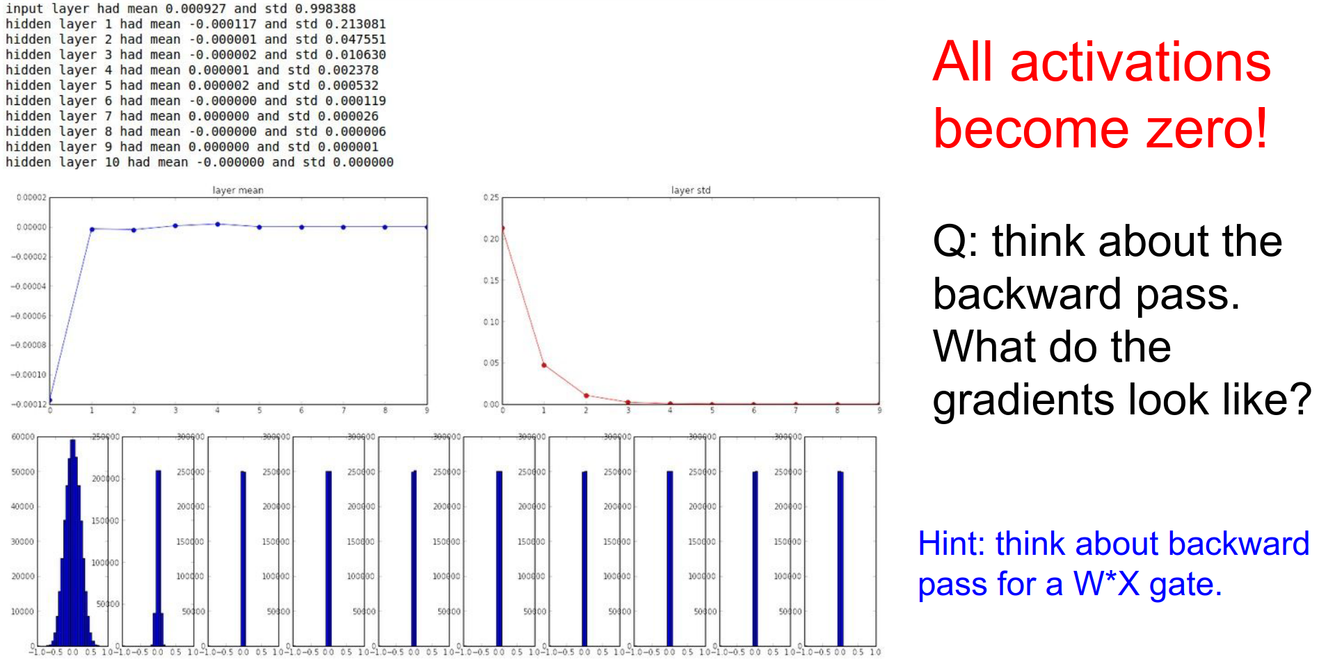
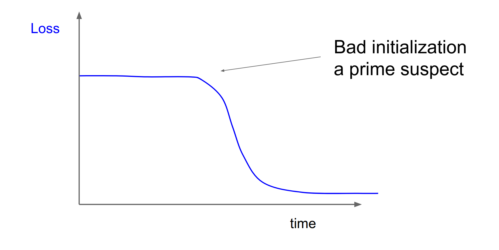
As data flows through the layers, it is multiplied by small numbers (0.01). The activations quickly shrink to zero.

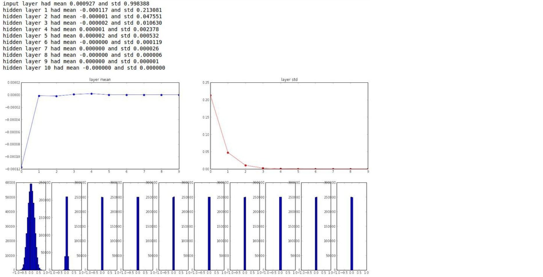
Why is this bad? During backpropagation, the gradient on the weights is \(X \times dL/df\). If the input \(X\) (the activation from the previous layer) is tiny, the gradient will be tiny. The network will not learn.

Large Random Numbers

What if we use larger weights? W = 1.0 * np.random.randn(D, H).

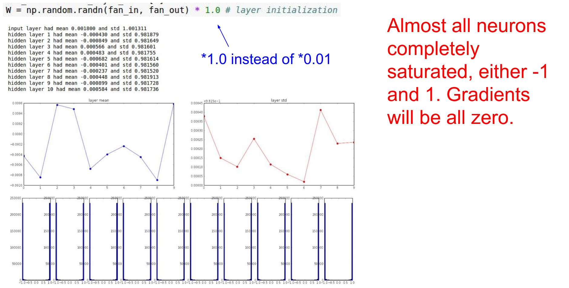
Now the neurons saturate. Tanh outputs become -1 or +1. The gradients become zero. The network does not learn.

Xavier Initialization

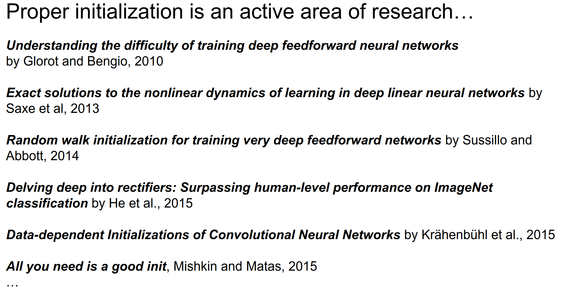
We want the variance of the input to be the same as the variance of the output. Glorot and Bengio (2010) derived a formula for this: W = np.random.randn(fan_in, fan_out) / np.sqrt(fan_in)

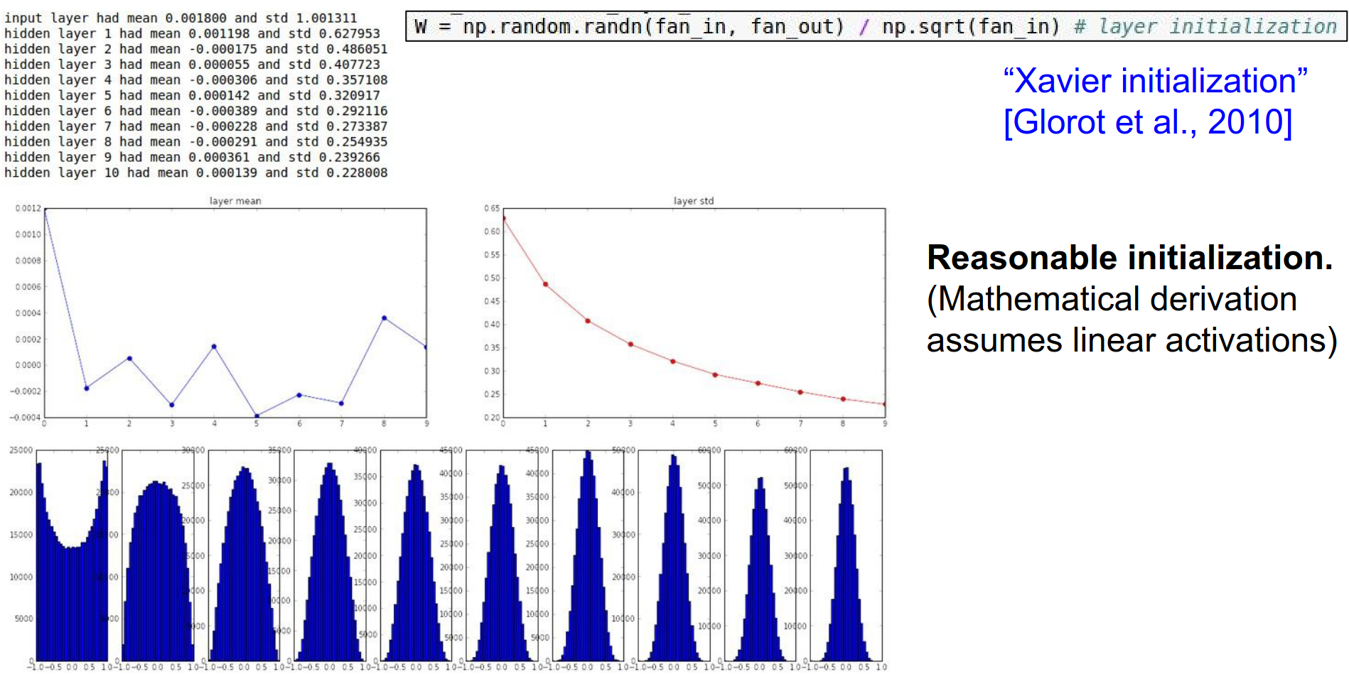
This keeps the activations well-scaled across many layers.

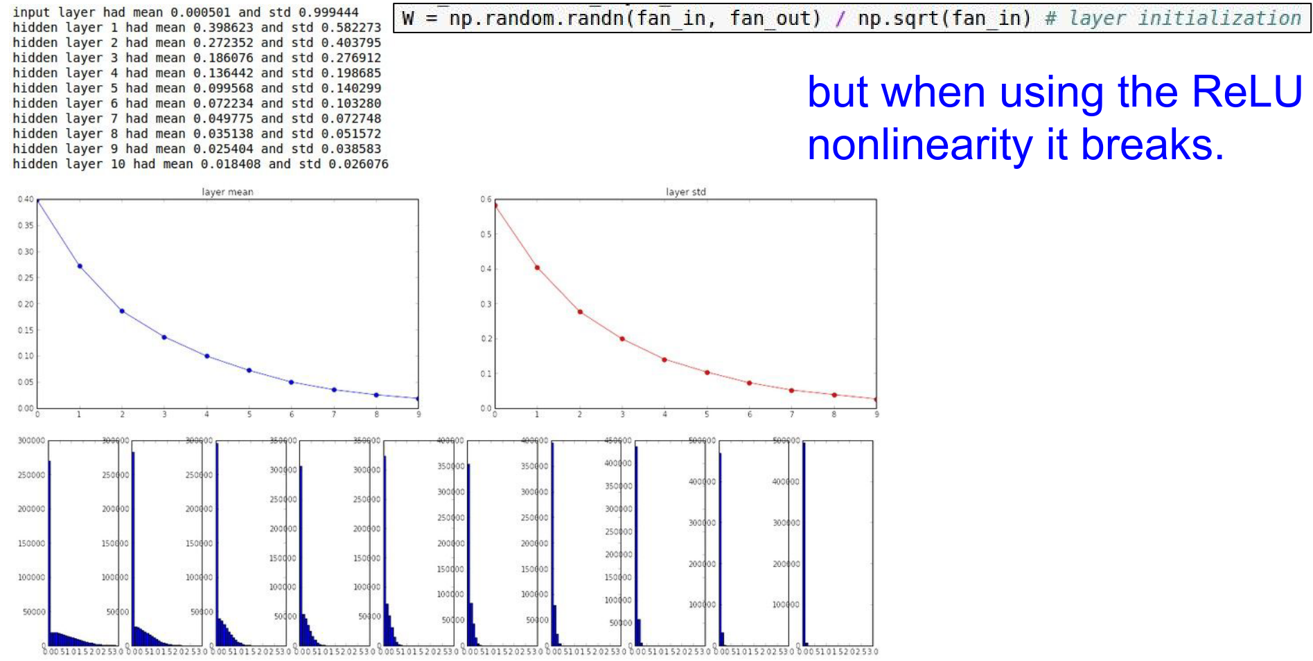
However, this derivation assumes linear activations. If we use ReLU, it breaks. ReLU kills half the variance (sets negative values to 0).

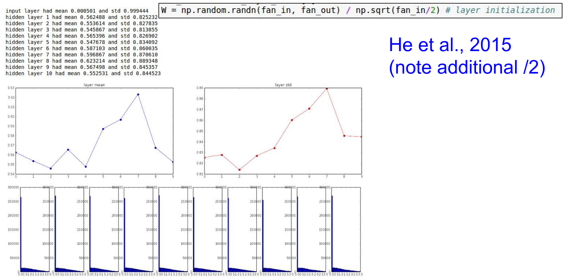
He Initialization

He et al. (2015) corrected this for ReLU by adding a factor of 2. W = np.random.randn(fan_in, fan_out) / np.sqrt(fan_in / 2)

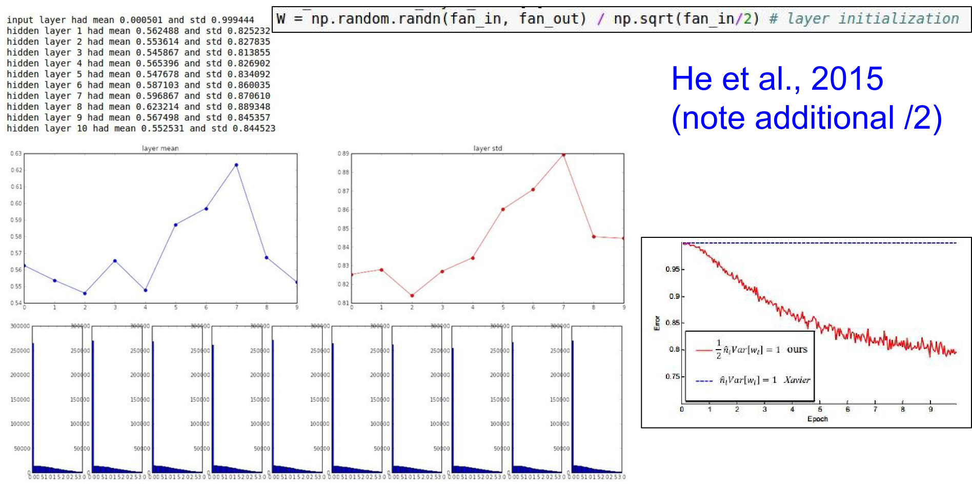
This is the current standard for initializing ReLU networks.

---

Batch Normalization

PS: This is explained in more detail in assignment 2.

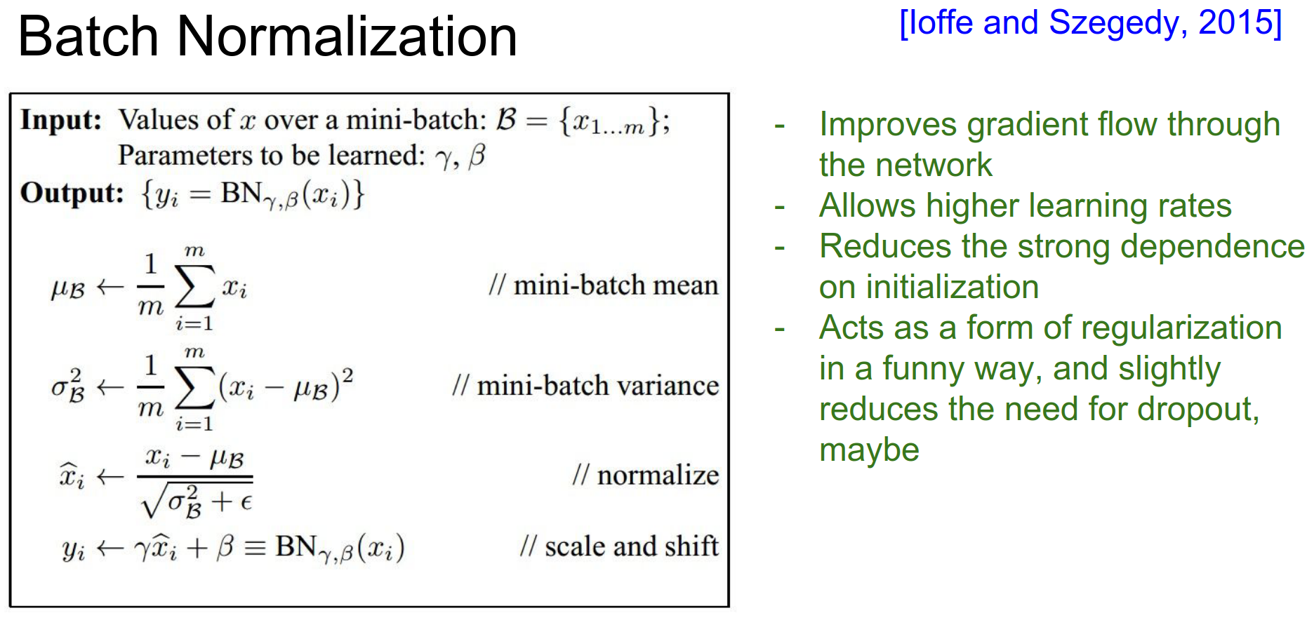
Batch Normalization (Ioffe & Szegedy, 2015) is a technique to explicitly force the activations to be unit gaussian throughout the network.

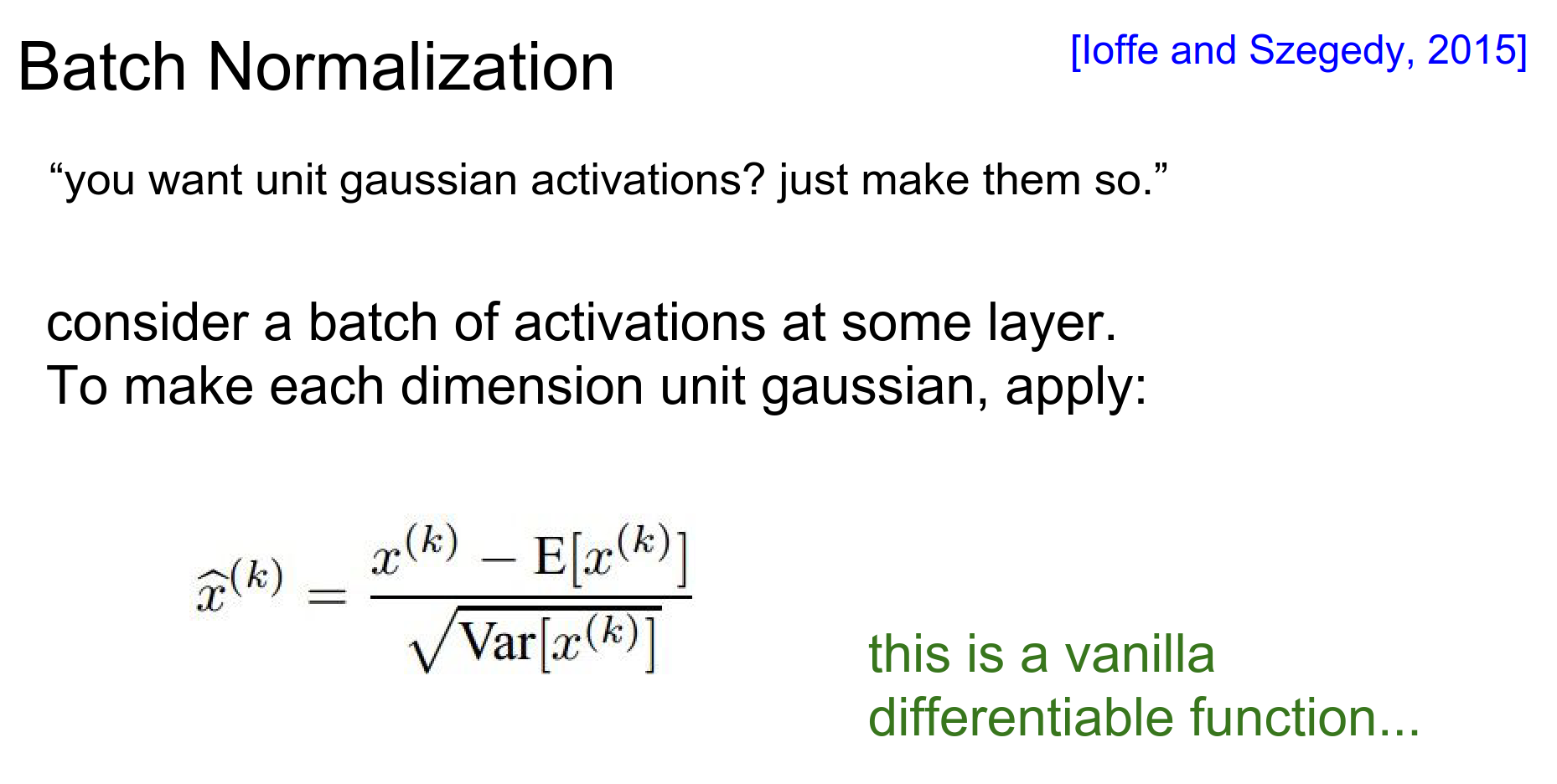
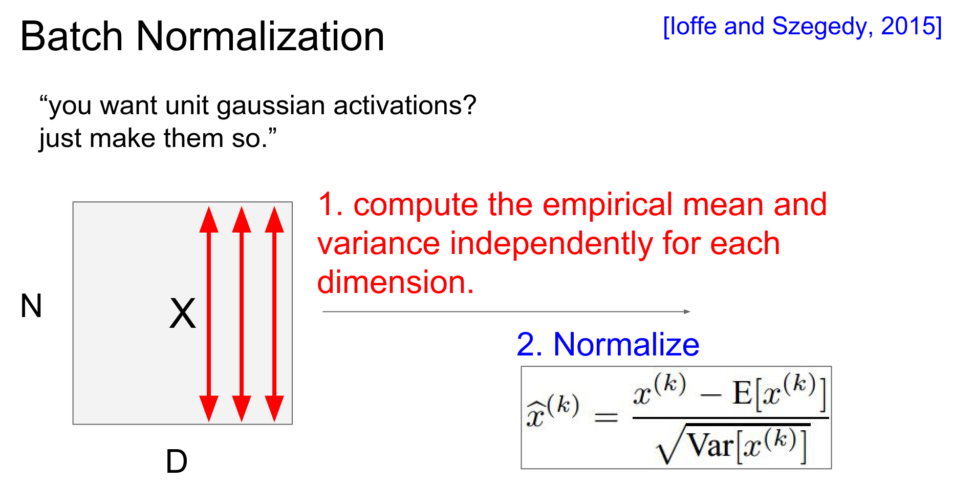
The Idea: For each feature dimension, compute the mean and variance over the current mini-batch, then normalize.

\[\hat{x} = \frac{x - \mu}{\sqrt{\sigma^2 + \epsilon}}\]

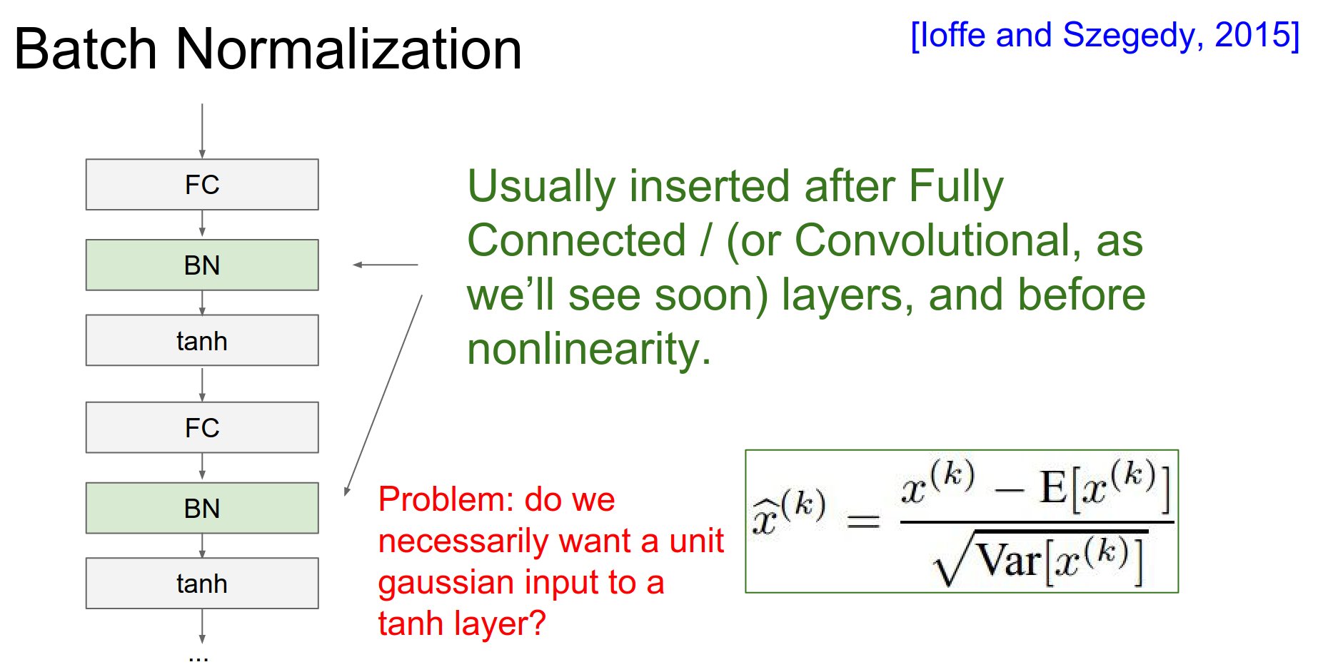
We typically insert this layer after the Fully Connected or Convolutional layer, and before the non-linearity.

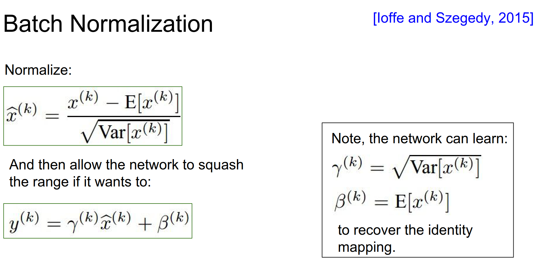
However, we don't want to constrain the network too much. We add learnable parameters \(\gamma\) (scale) and \(\beta\) (shift) so the network can learn to undo the normalization if it needs to.

\[y = \gamma \hat{x} + \beta\]

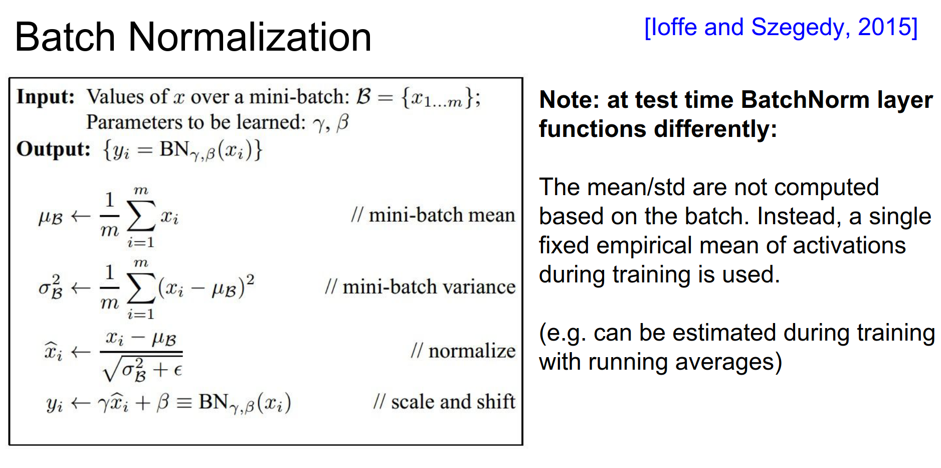
At Test Time: We don't use the batch mean/variance. Instead, we use a running average of mean/variance collected during training.

Benefits:

• Reduces sensitivity to initialization.

• Allows higher learning rates.

• Acts as a regularizer.

It is good thing to use. But there is a runtime penalty.

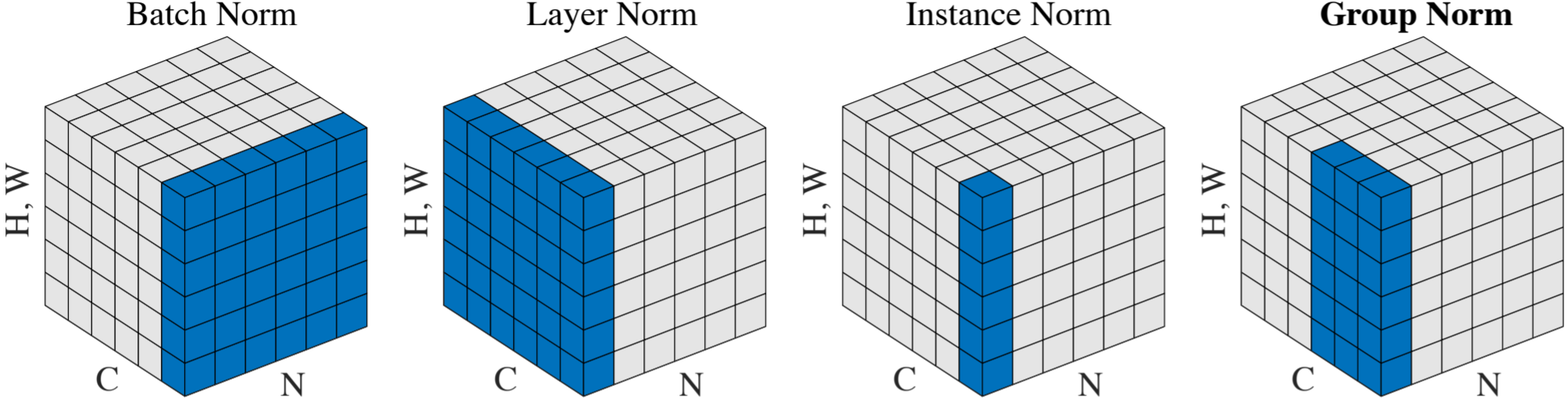
Layer Normalization: A related technique is Layer Normalization, which normalizes across the features for a single example, rather than across the batch. This is useful for RNNs or when batch sizes are small.

---

Babysitting the Learning Process

Now we look at the practical steps of monitoring training.

Step 1: Preprocessing: Zero-center your data.

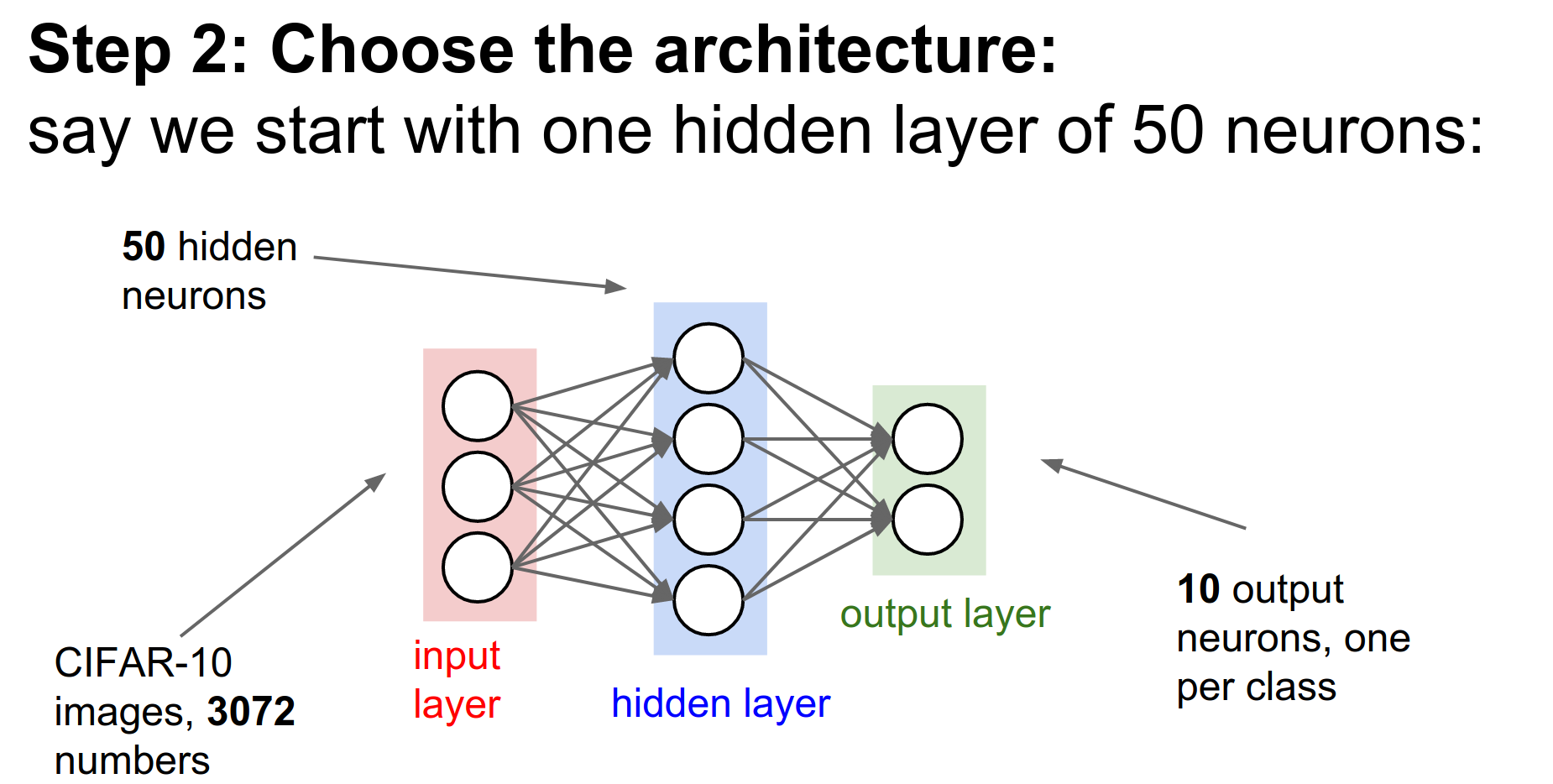
Step 2: Architecture: Choose your architecture (e.g., 2-layer net, 50 hidden neurons).

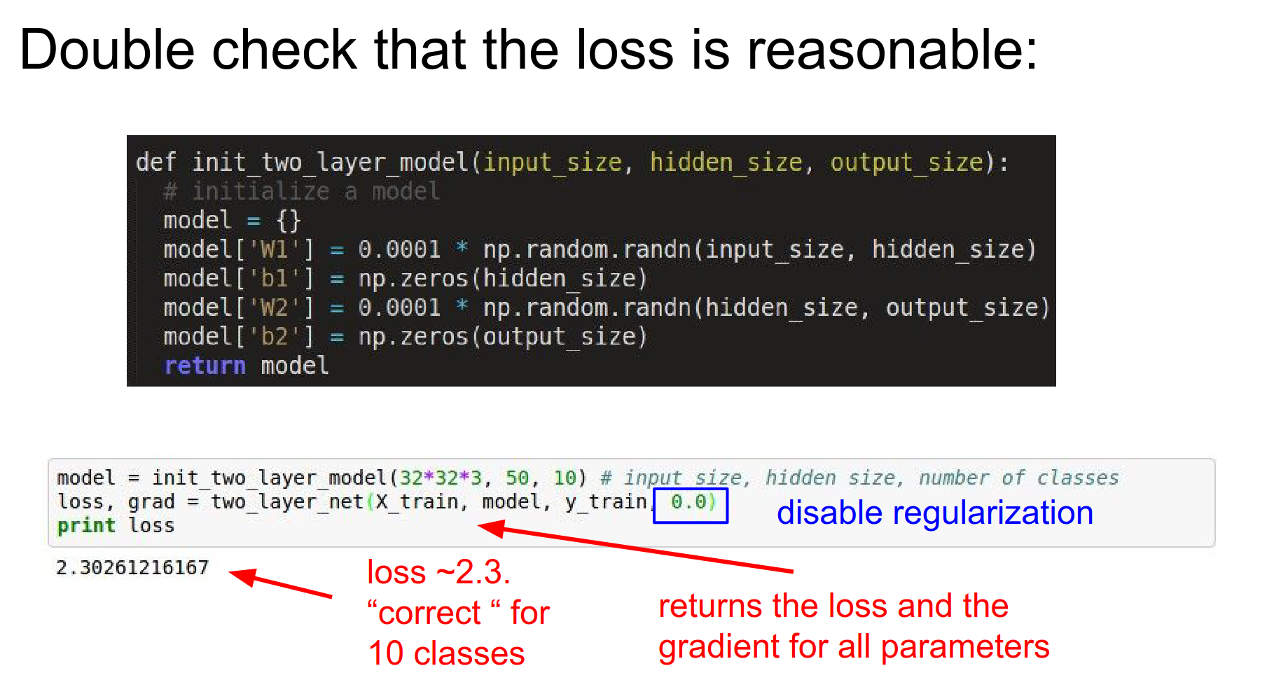
Step 3: Double Check the Loss: Disable regularization. The loss should be around \(-\log(1/C)\) where \(C\) is the number of classes. For CIFAR-10 (\(C=10\)), loss should be \(\approx 2.3\).

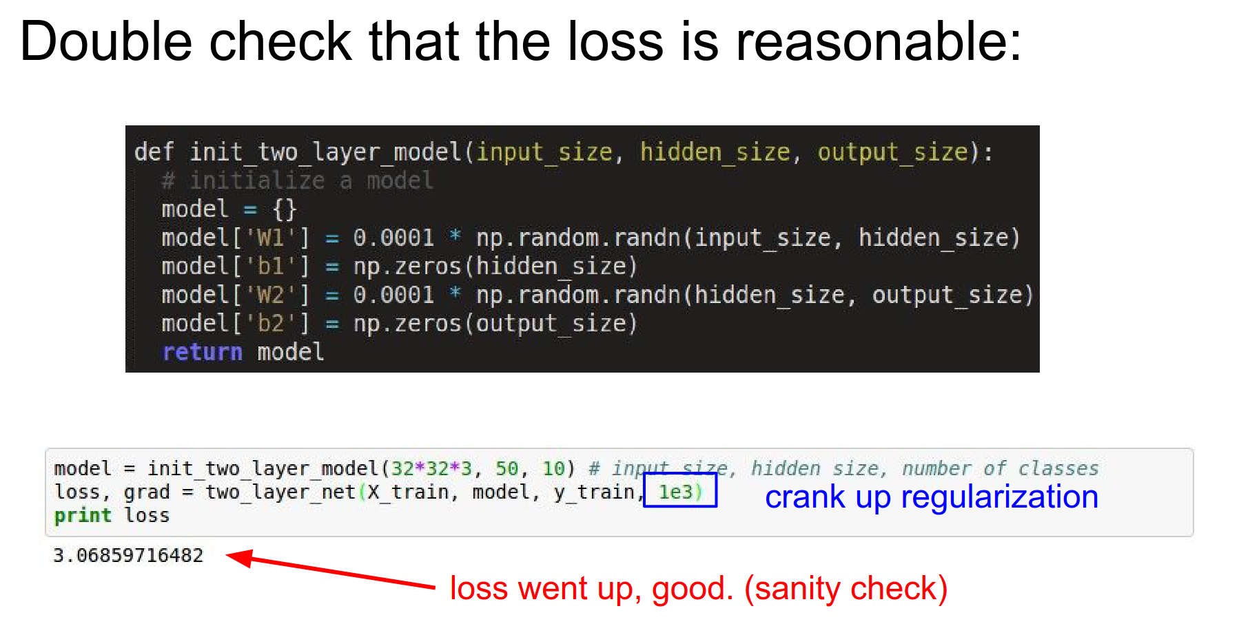
If you add regularization, the loss should go up.

Step 4: Sanity Check (Overfit Small Data): Take a tiny subset of data (e.g., 20 examples). Turn off regularization. Train. You should be able to get 100% accuracy and loss of 0.

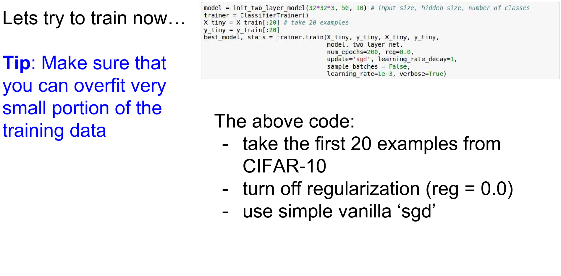
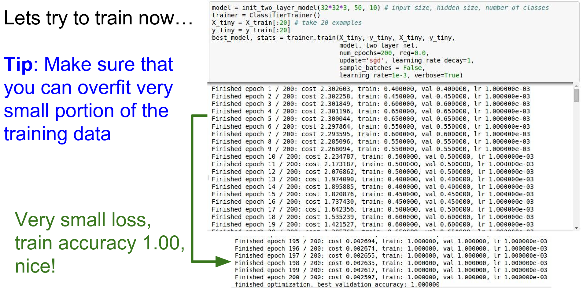
If you can't overfit a small dataset, your model is broken.

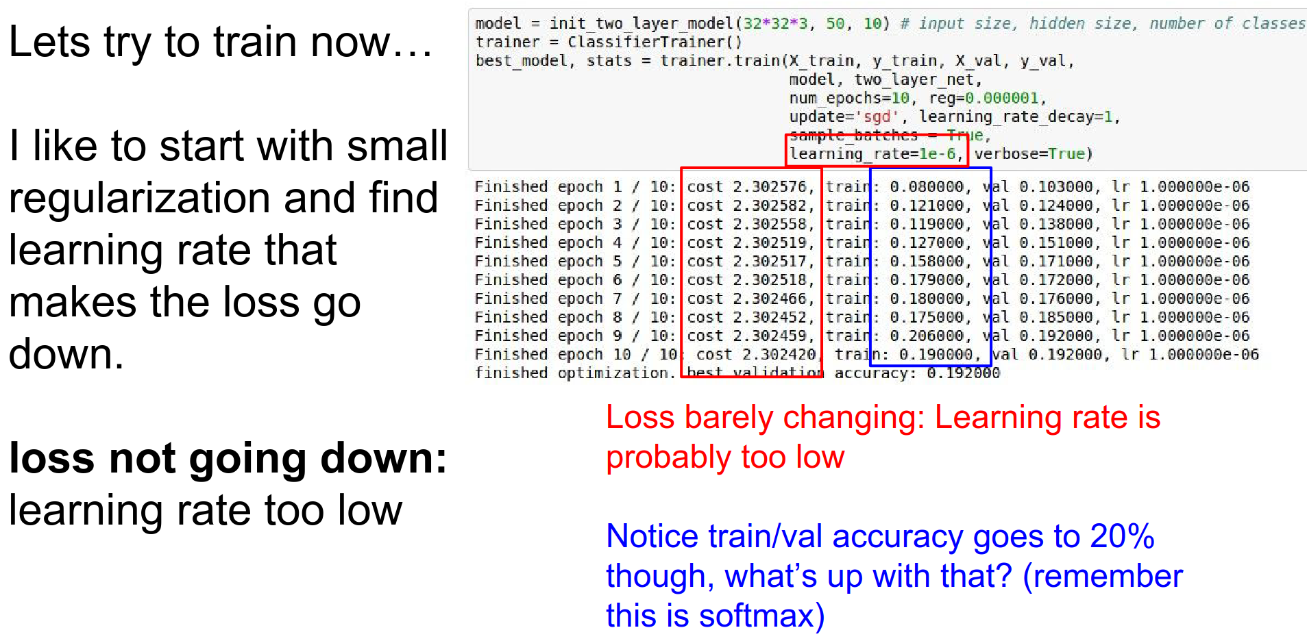
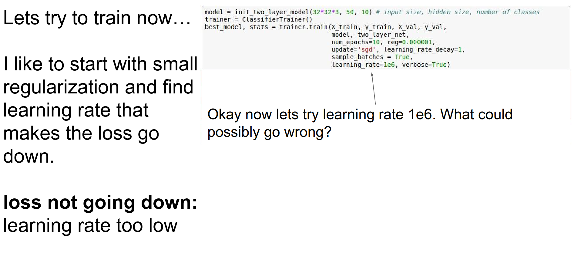
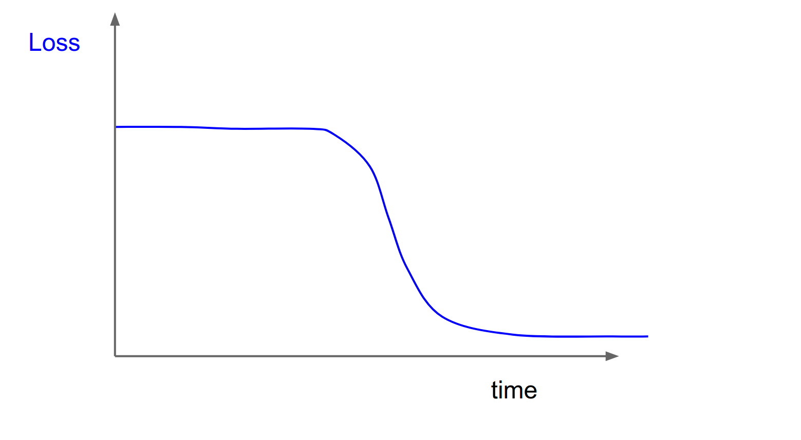
Step 5: Find Learning Rate: Now use the full dataset (with small regularization). Start with a small learning rate.

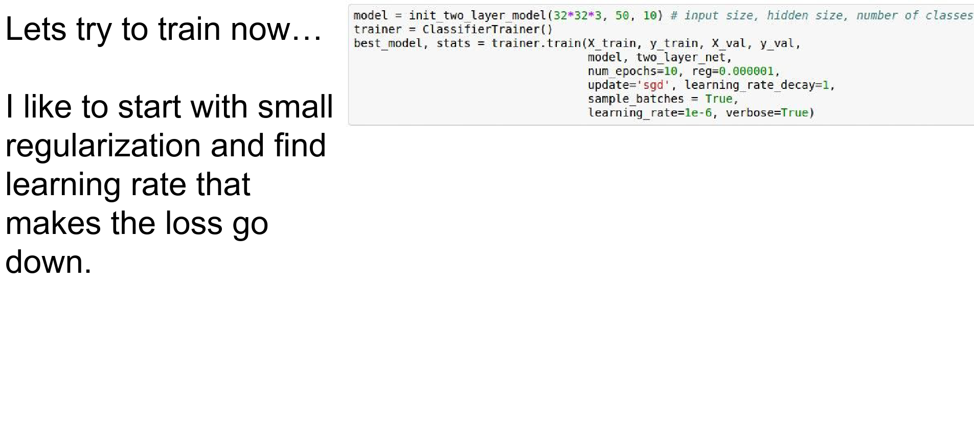
If the loss doesn't go down, the learning rate is too low.

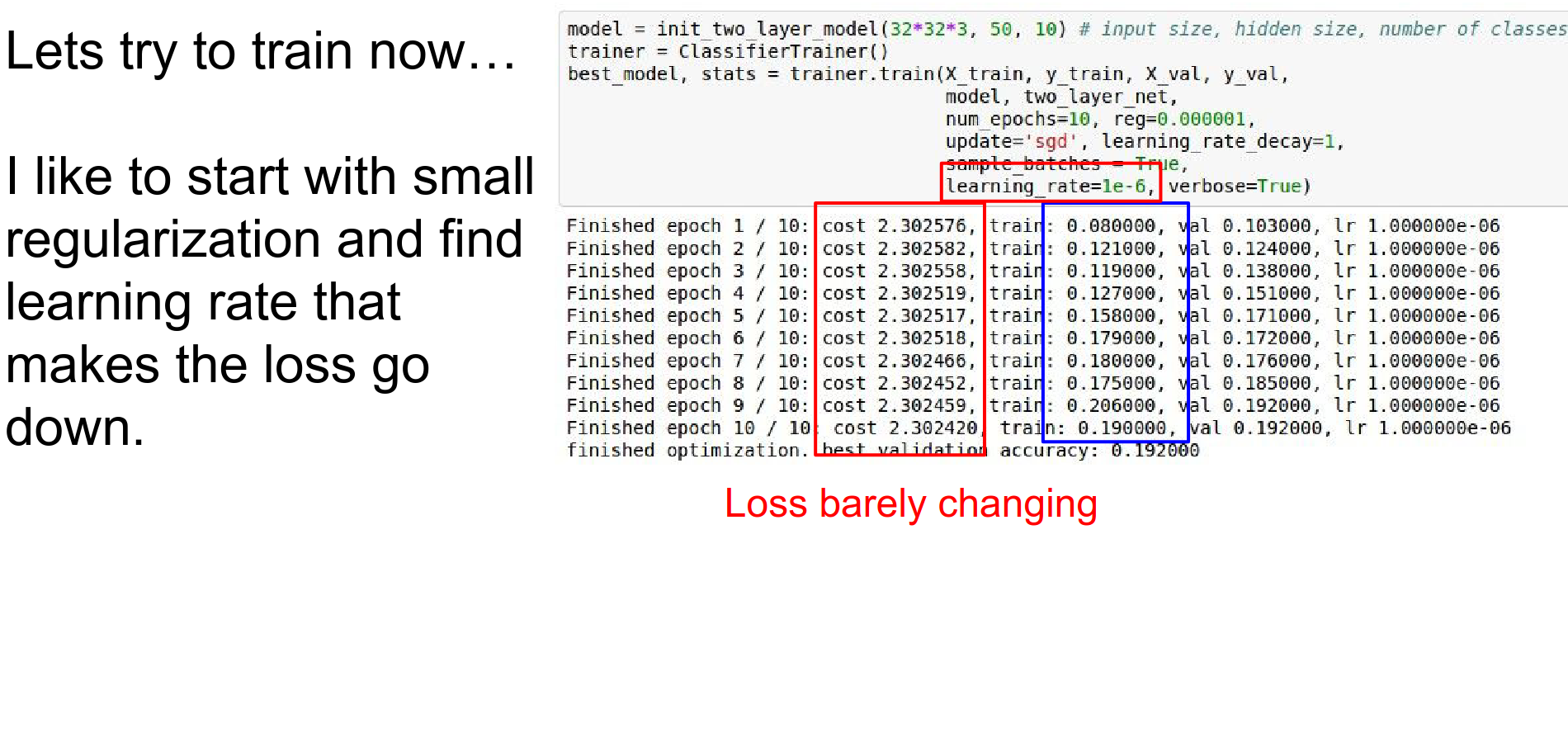
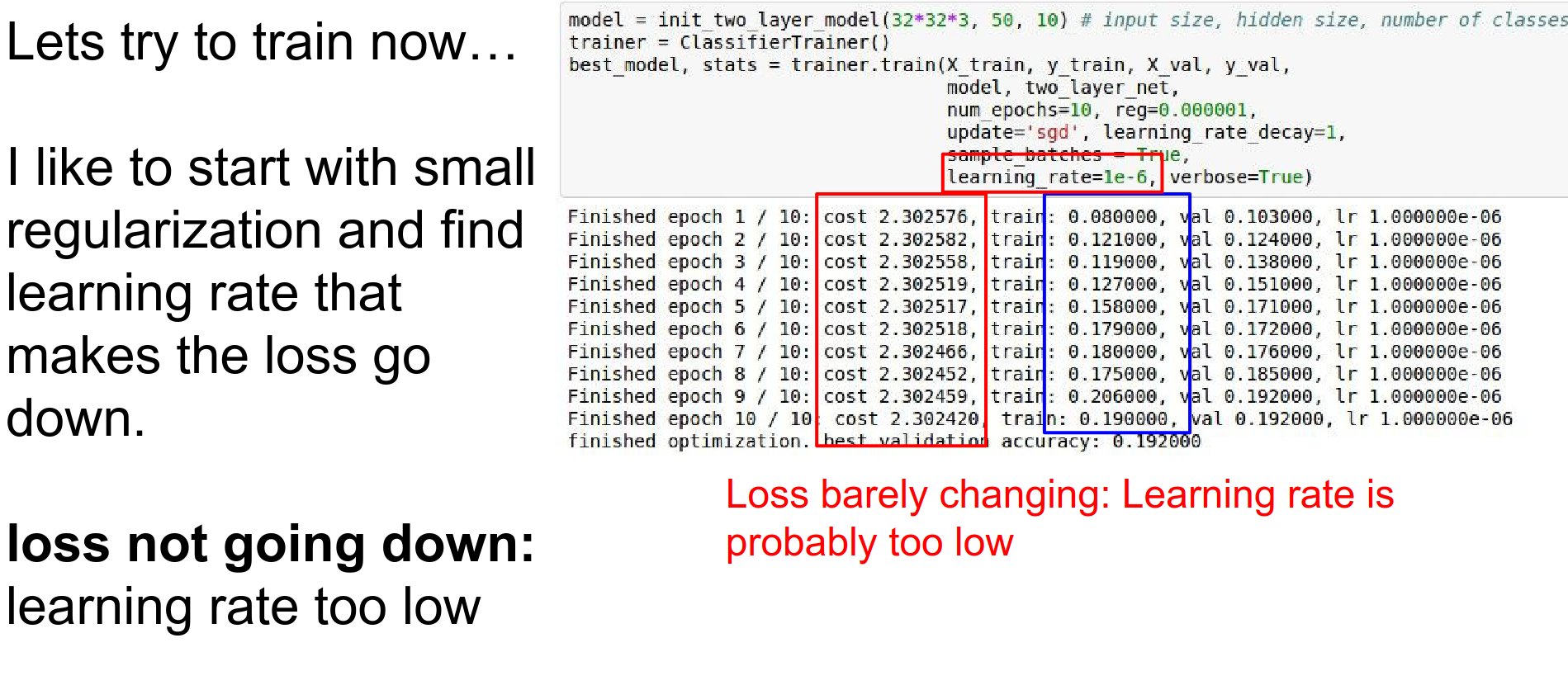
Notice that loss barely changes, but accuracy jumps? This is because weights are shifting slightly to make correct scores just barely higher.

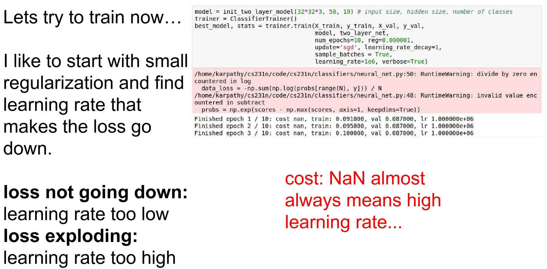
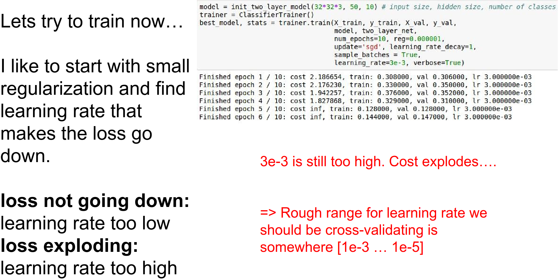
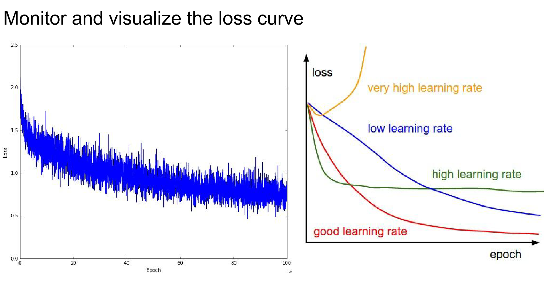
If the learning rate is too high, the loss explodes (NaN).

You want to find a learning rate that is "just right" (roughly in the range [\(1e^{-3}\), \(1e^{-5}\)]).

---

Hyperparameter Optimization

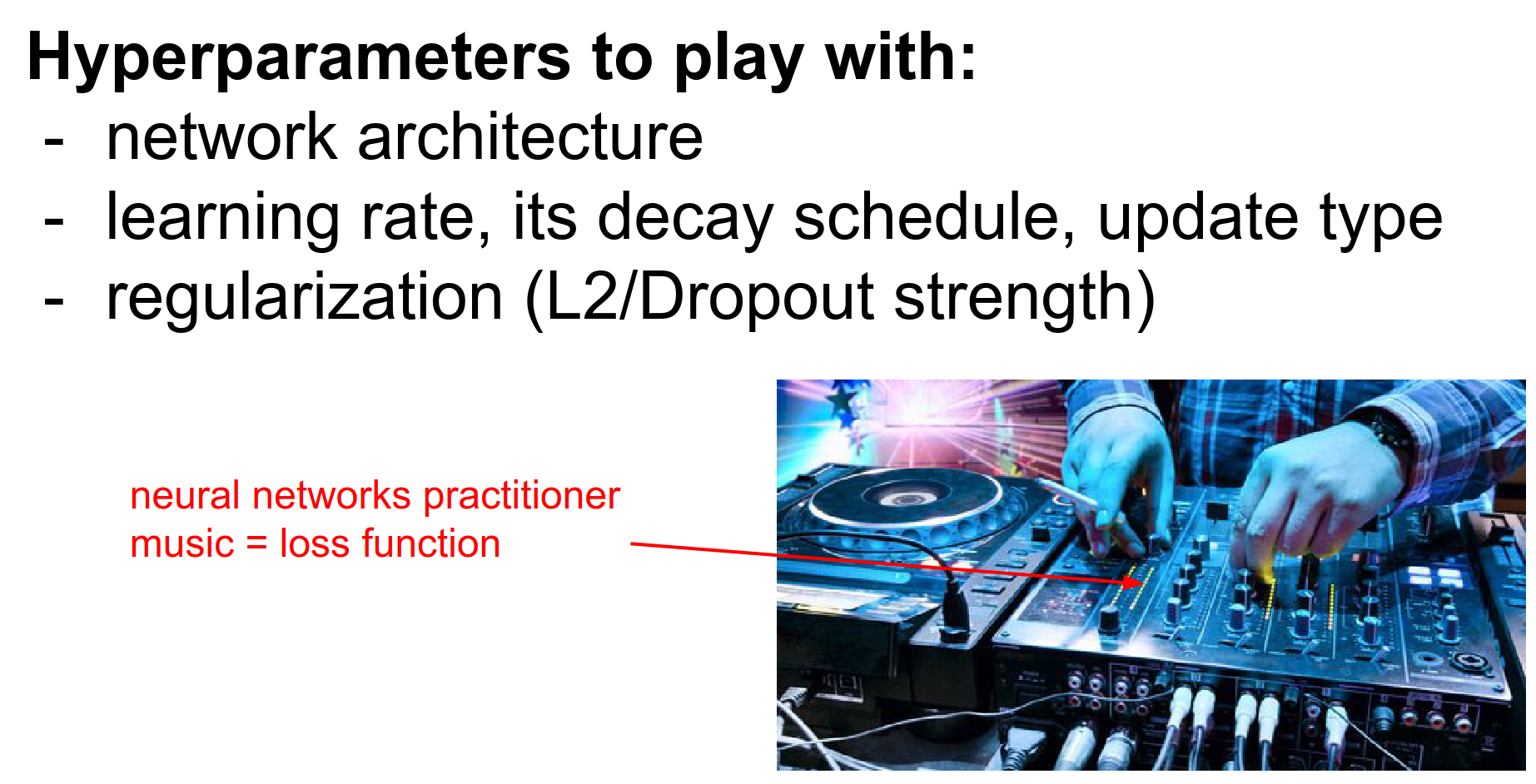
We need to find the best hyperparameters (Learning Rate, Regularization, Dropout, etc.).

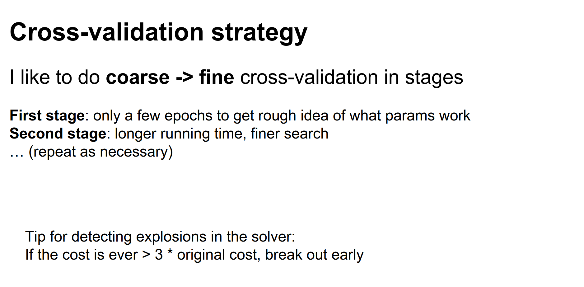
Strategy: Coarse to Fine First, search a wide range for a few epochs.

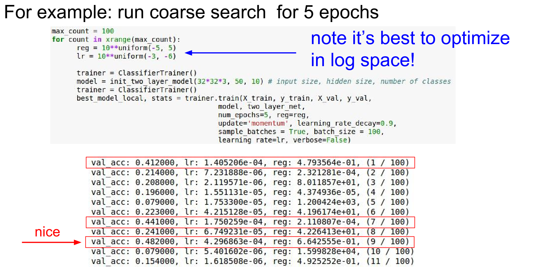
Tip: Optimize in Log Space. Learning rates and regularization strengths are multiplicative. Sample exponents uniformly from a range. 10 ** uniform(-3, -6)

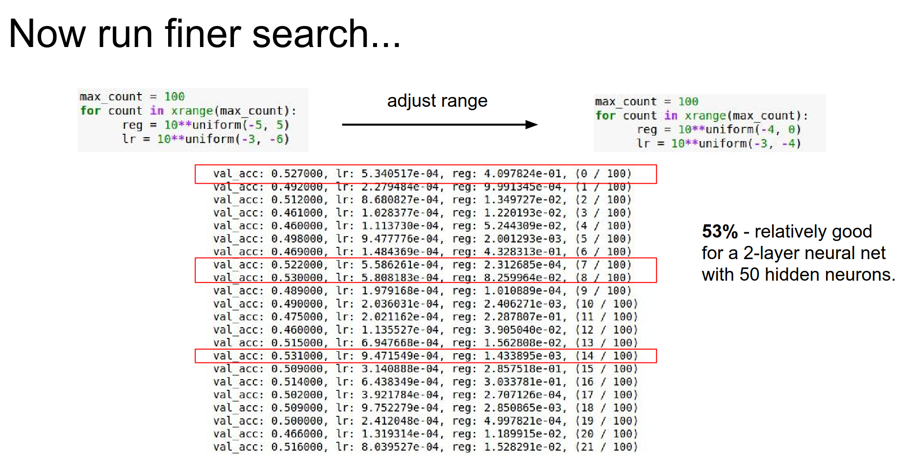
Once you find a good region, narrow the search and run for longer.

Random Search vs. Grid Search Always use Random Search.

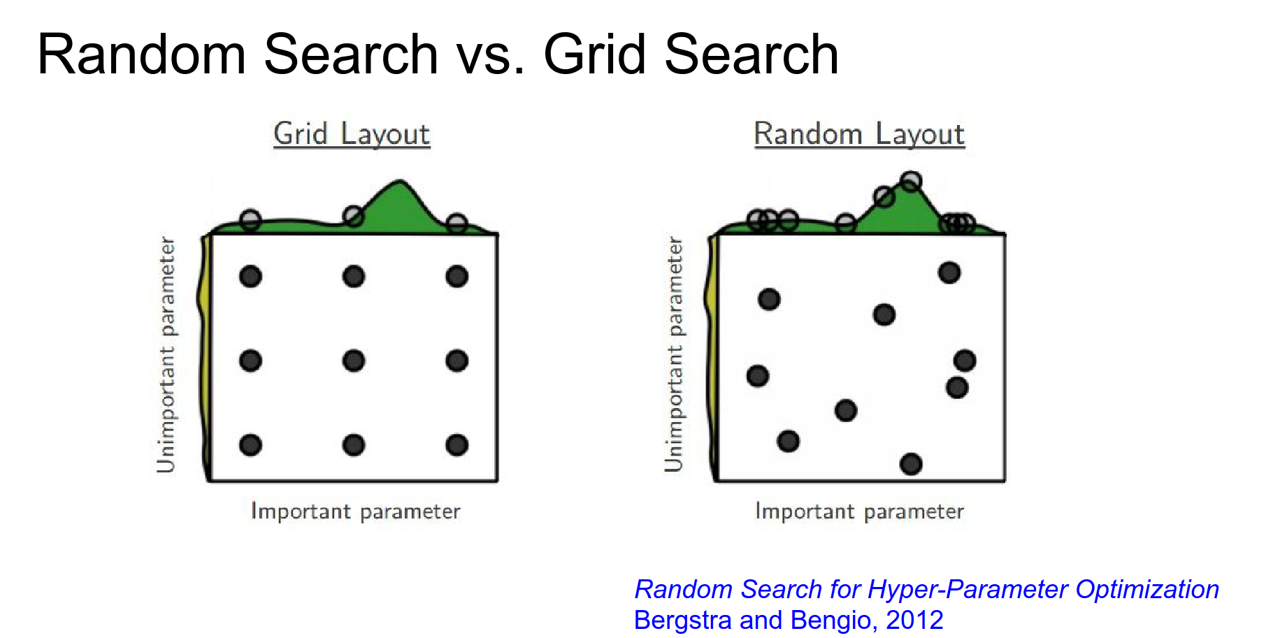
Grid search is inefficient because some hyperparameters are more important than others. Random search explores more unique values for the important parameters.

Visualizing Results Plot your results.

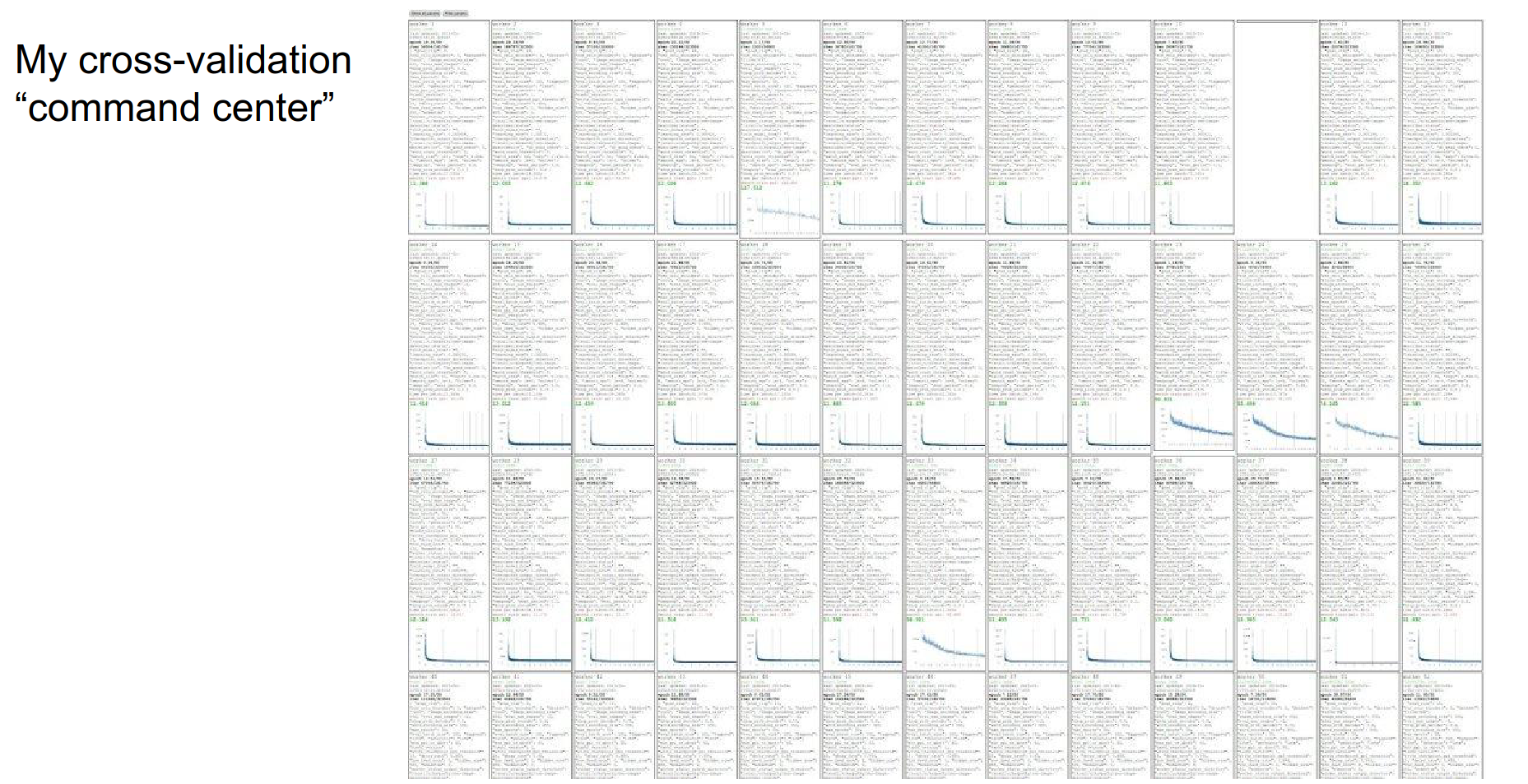
You cannot spray and pray :).

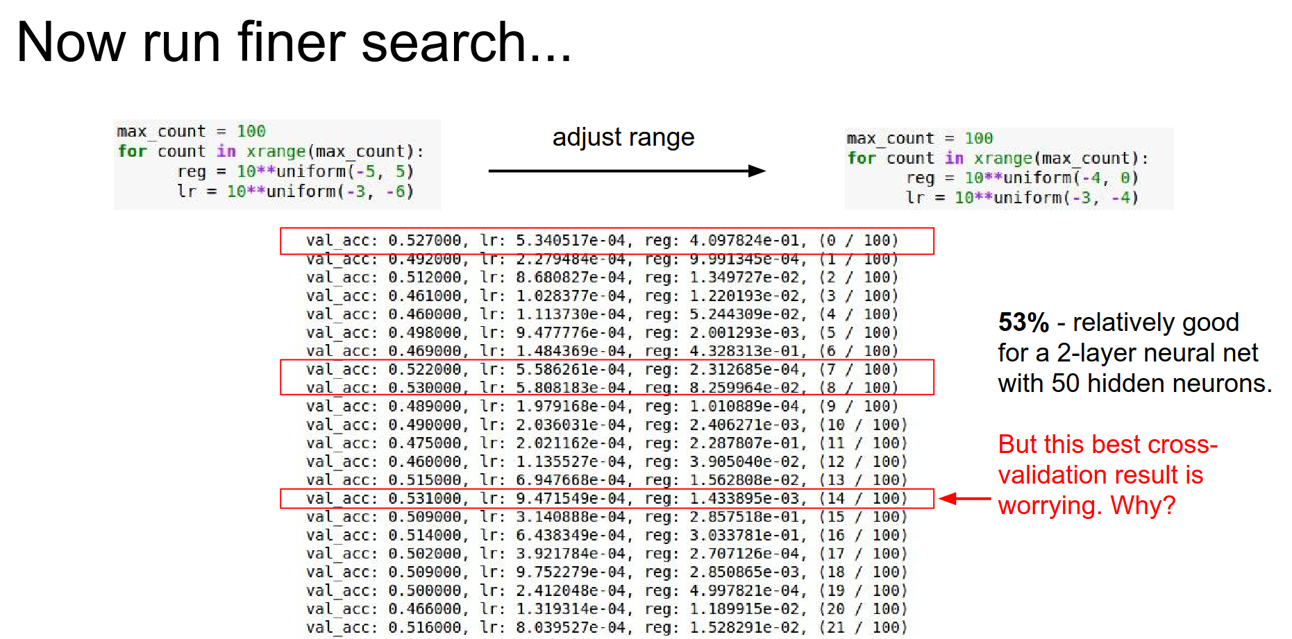
If your best results are on the edge of your search range, you need to shift the range!

Evaluation

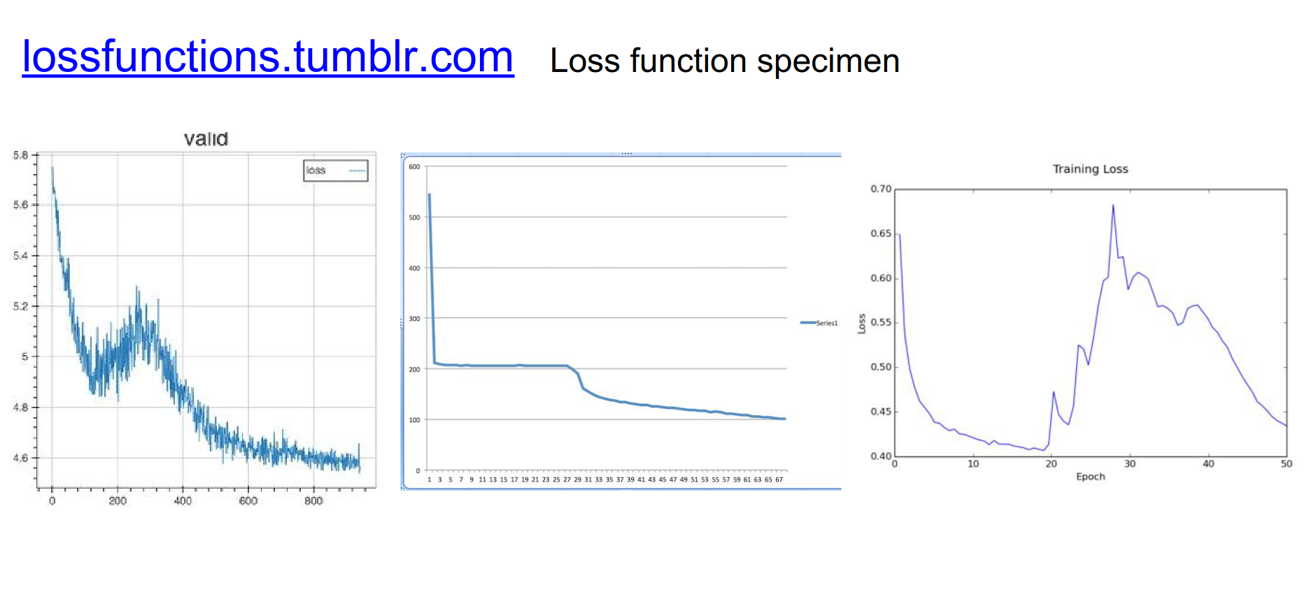
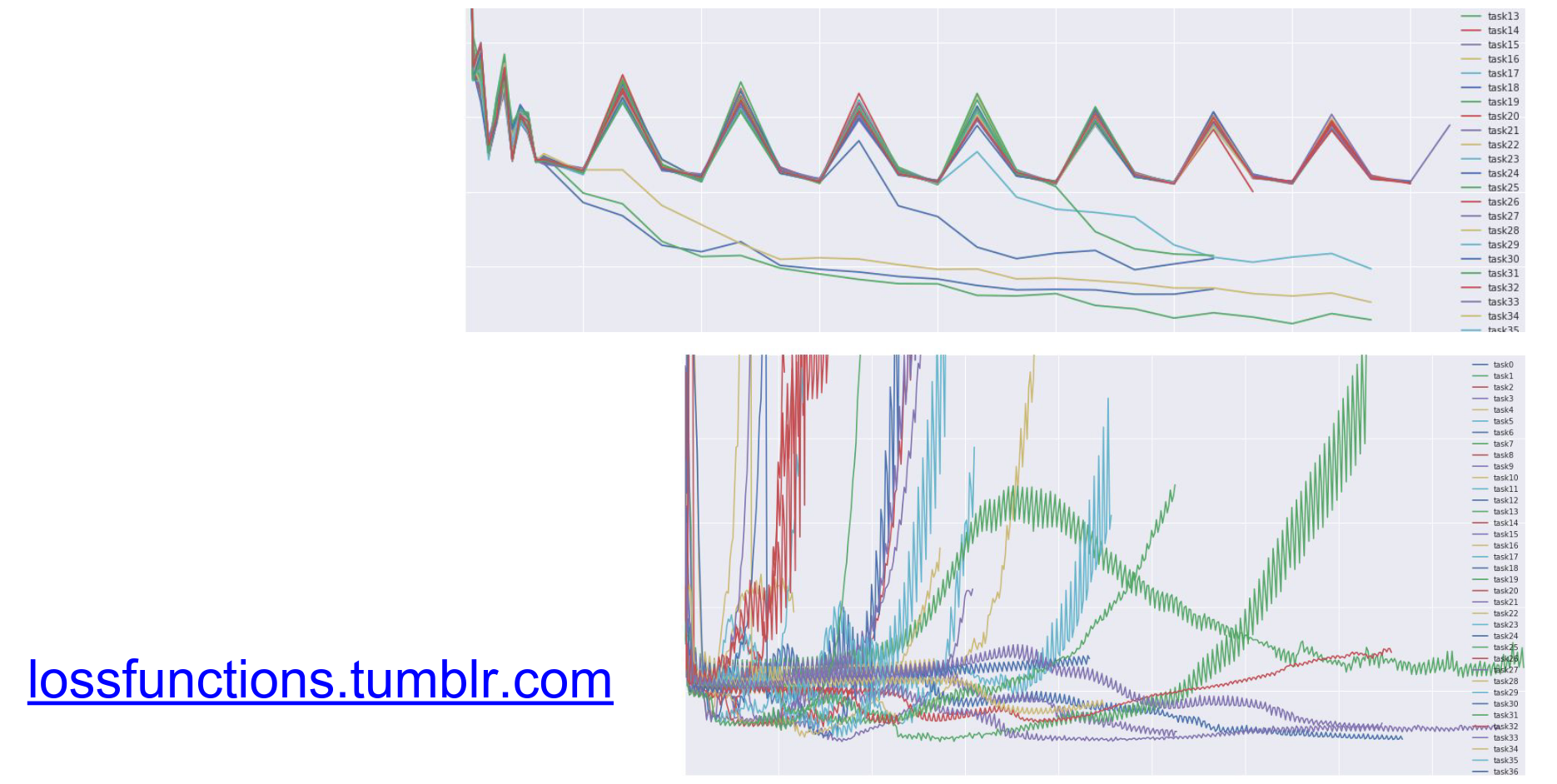
Monitor your loss curves.

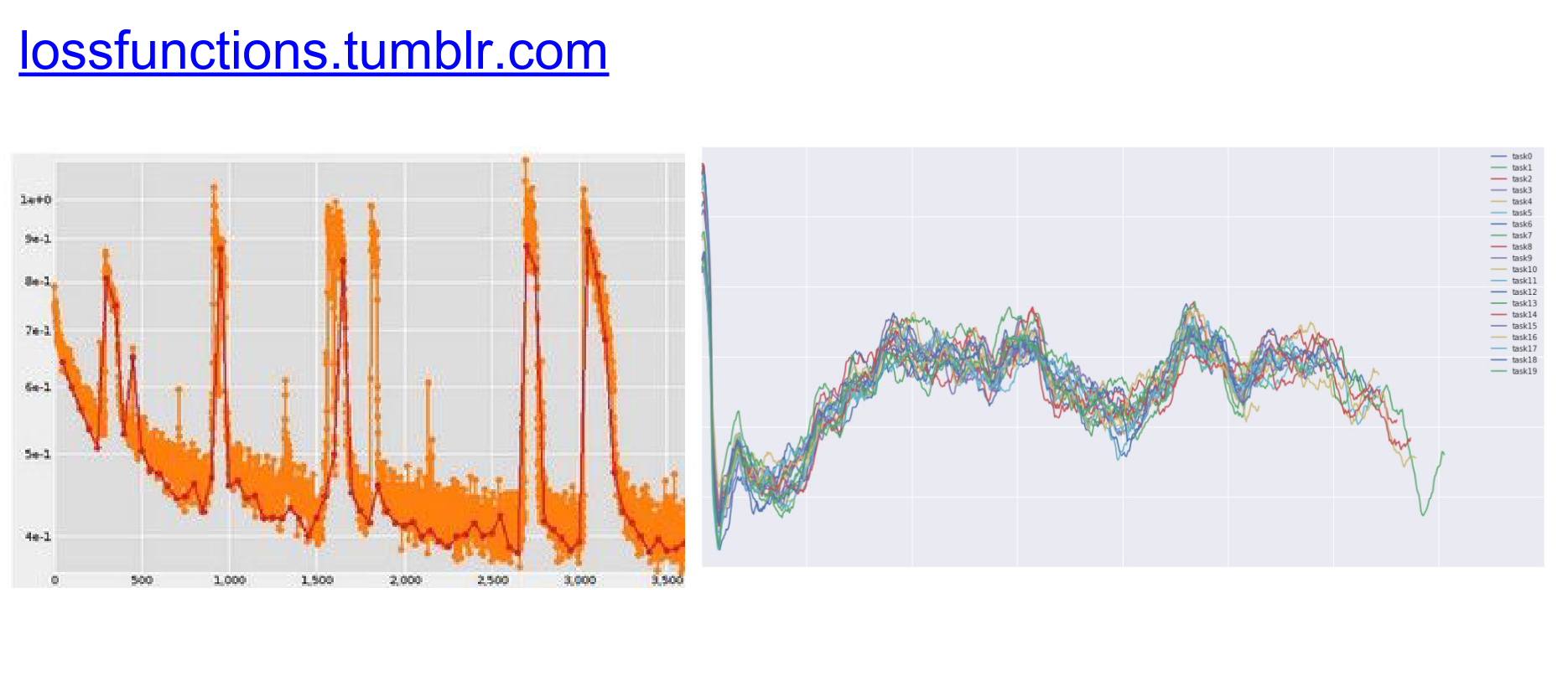
(Check out lossfunctions.tumblr.com for examples of loss curves).

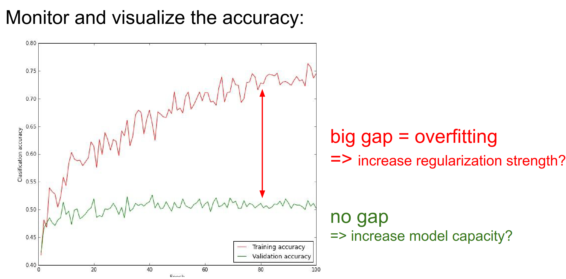
Monitor the gap between training and validation accuracy.

• Big gap = Overfitting (increase regularization).

• No gap = Underfitting (increase model capacity).

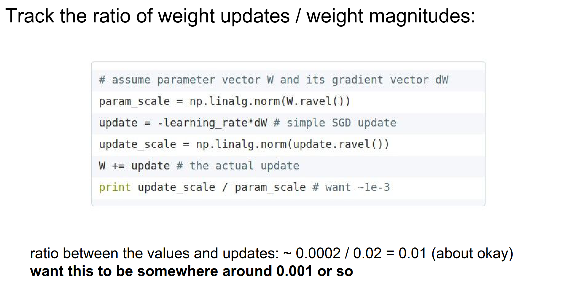
Weight:Update Ratio Track the ratio of the update magnitude to the weight magnitude. It should be around \(1e^{-3}\).

Summary

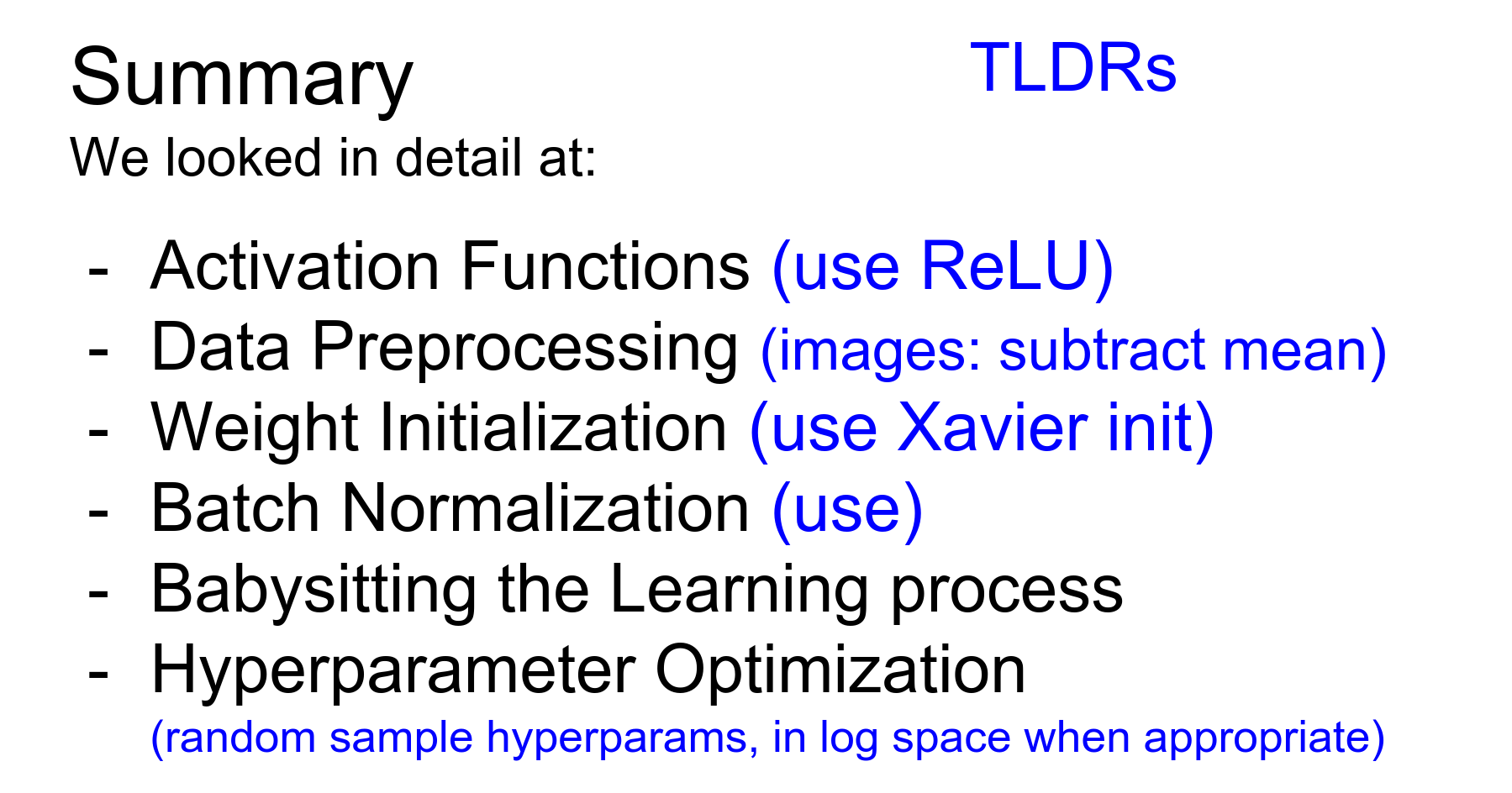
We have covered:

• Activation Functions (use ReLU).

• Data Preprocessing (zero-center).

• Weight Initialization (use Xavier/He).

• Batch Normalization (use it).

• Hyperparameter Optimization (random search in log space).

In the next lecture, we will continue with parameter updates and more advanced training techniques.