6. Training Neural Networks Part 2
Part of CS231n Winter 2016
Lecture 6: Training Neural Networks, Part 2
By the end of the assignment, you will have a good understanding of all the low-level details of how a ConvNet classifies images.
I am so excited! Here is the Assignment link again.
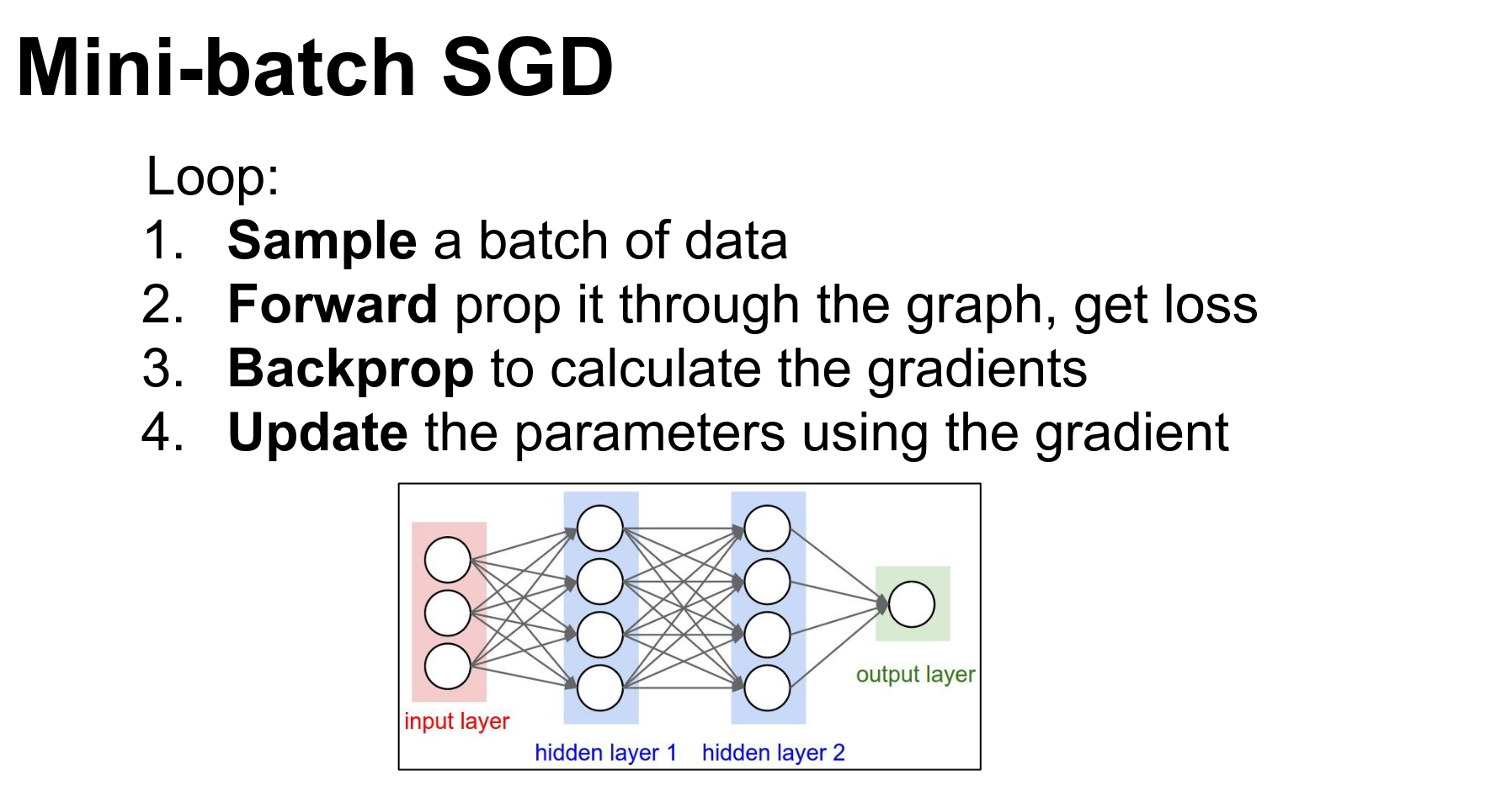
Training a ConvNet is a four-step process.
-
Loss: Tells us how well we are classifying at the moment.
-
Backpropagation: We backpropagate to compute the gradient on all the weights. This gradient tells us how we should nudge every single weight to make better classifications.
-
Update: We use the gradients to make a small nudge to the weights.
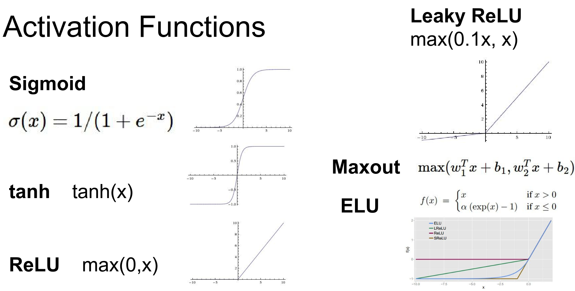
There is an entire zoo of activation functions available.
Activation Functions
If you do not use an activation function, your entire network will be a linear sandwich.
Your capacity is equal to that of just a linear classifier.
Activation functions are critical; they provide the non-linearity needed to fit your data.
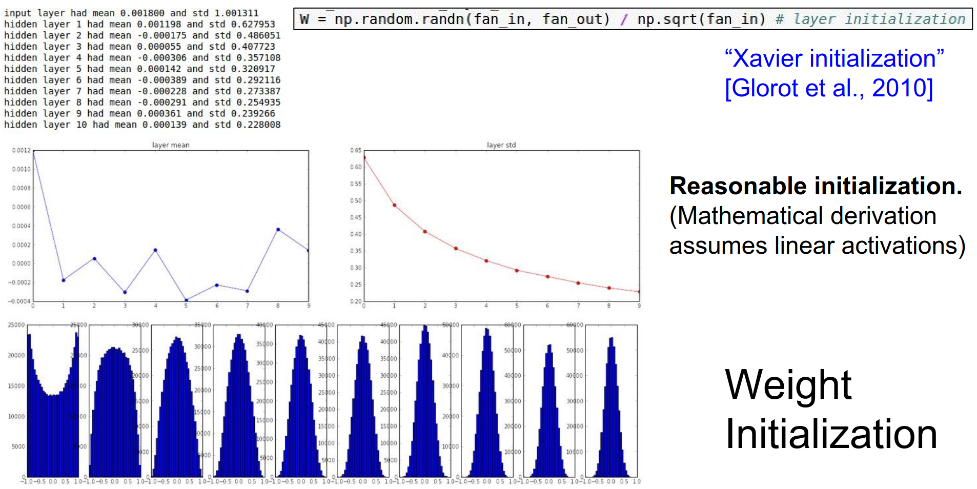
The problem here is: how should we start? Xavier initialization is a reasonable starting point.
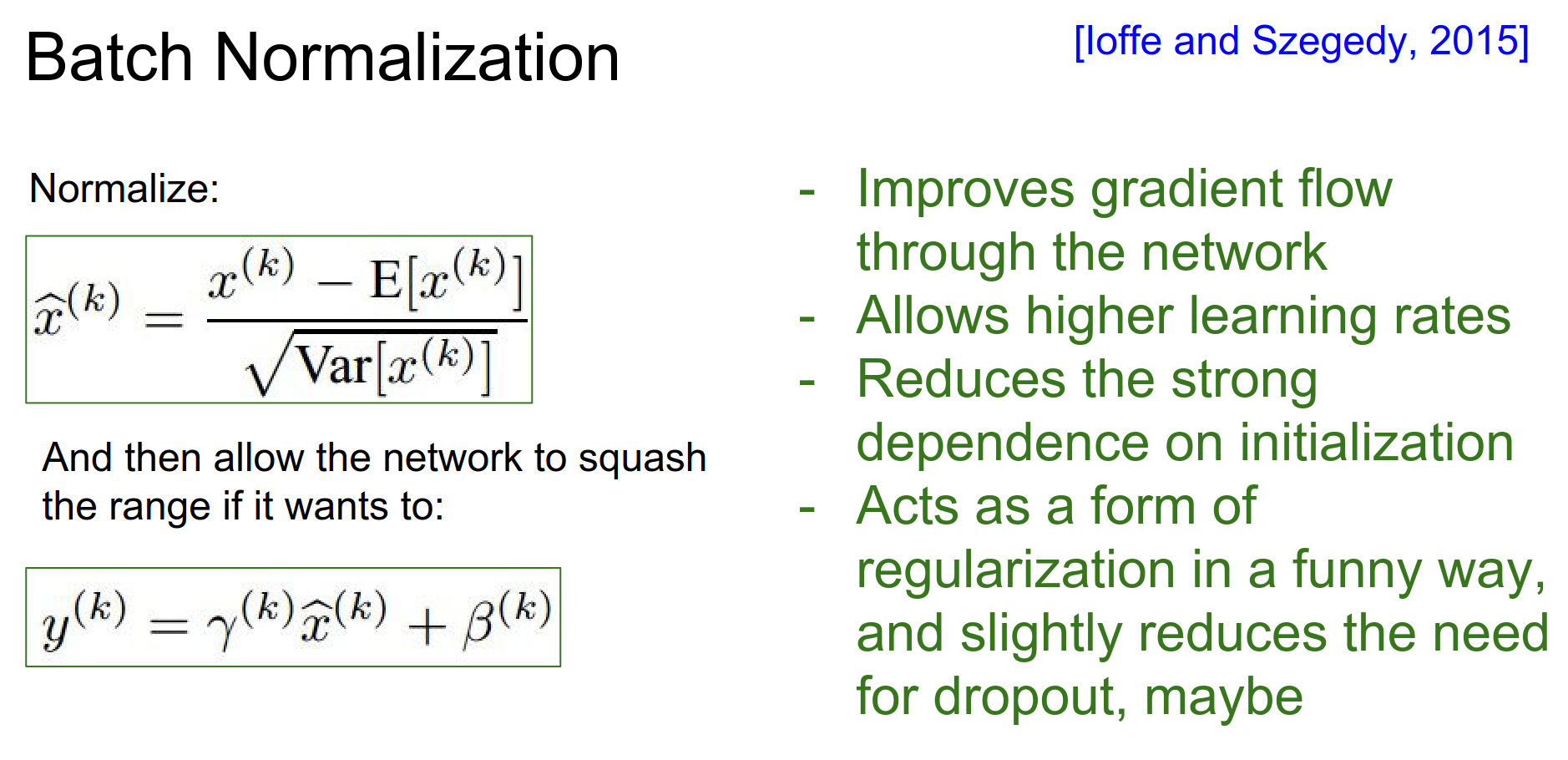
Batch Normalization (BN) gets rid of many headaches. It reduces the strong dependence on initialization.
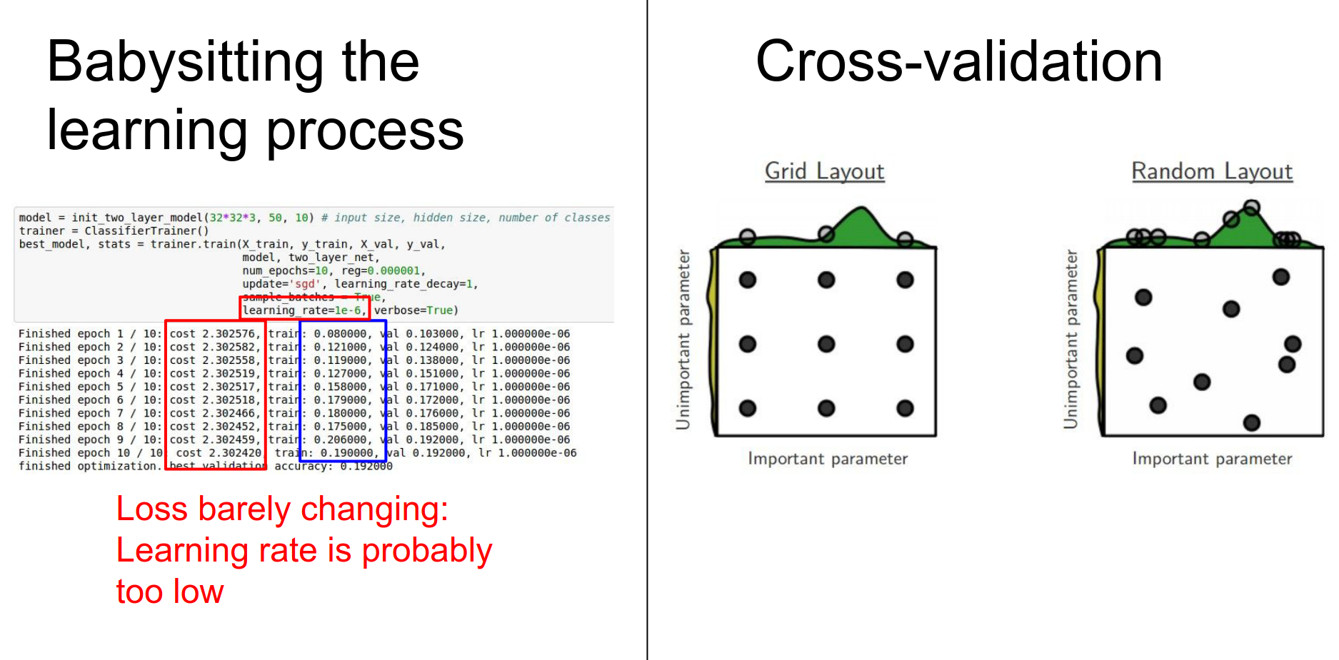
Here are some tips and tricks for babysitting the learning process.
Today's Agenda
The process looks like this:
- Loss: Tells us how well we are classifying at the moment.
- Backpropagation: We backpropagate to compute the gradient on all the weights. This gradient tells us how we should nudge every single weight to make better classifications.
- Update: We use the gradients to make a small nudge to the weights.
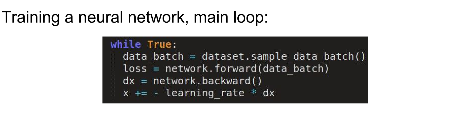
Parameter update is just gradient descent. Can we make it better?
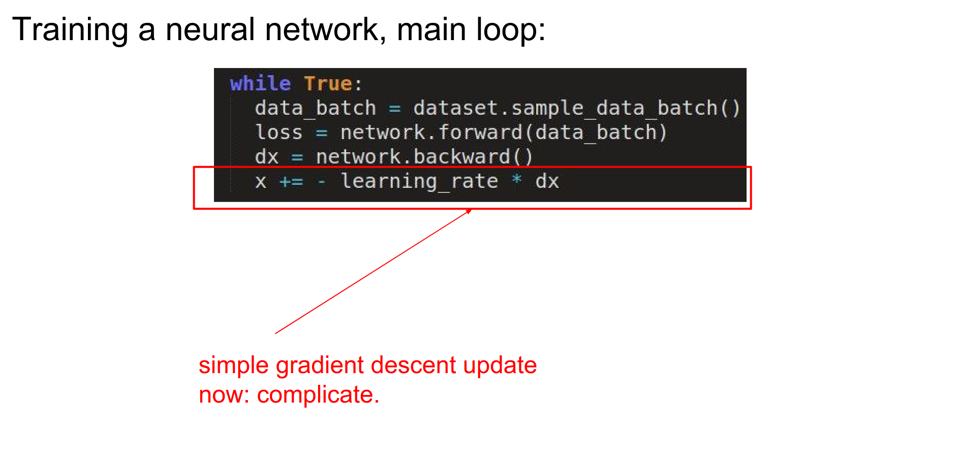
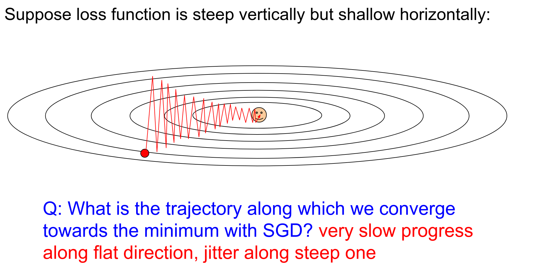
Stochastic Gradient Descent
The classic .gif is shown below. In practice, you rarely use vanilla SGD.
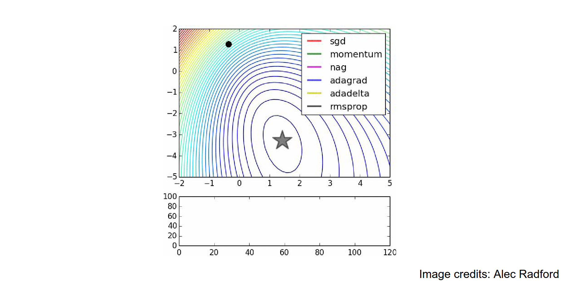
SGD is the slowest among all of them.
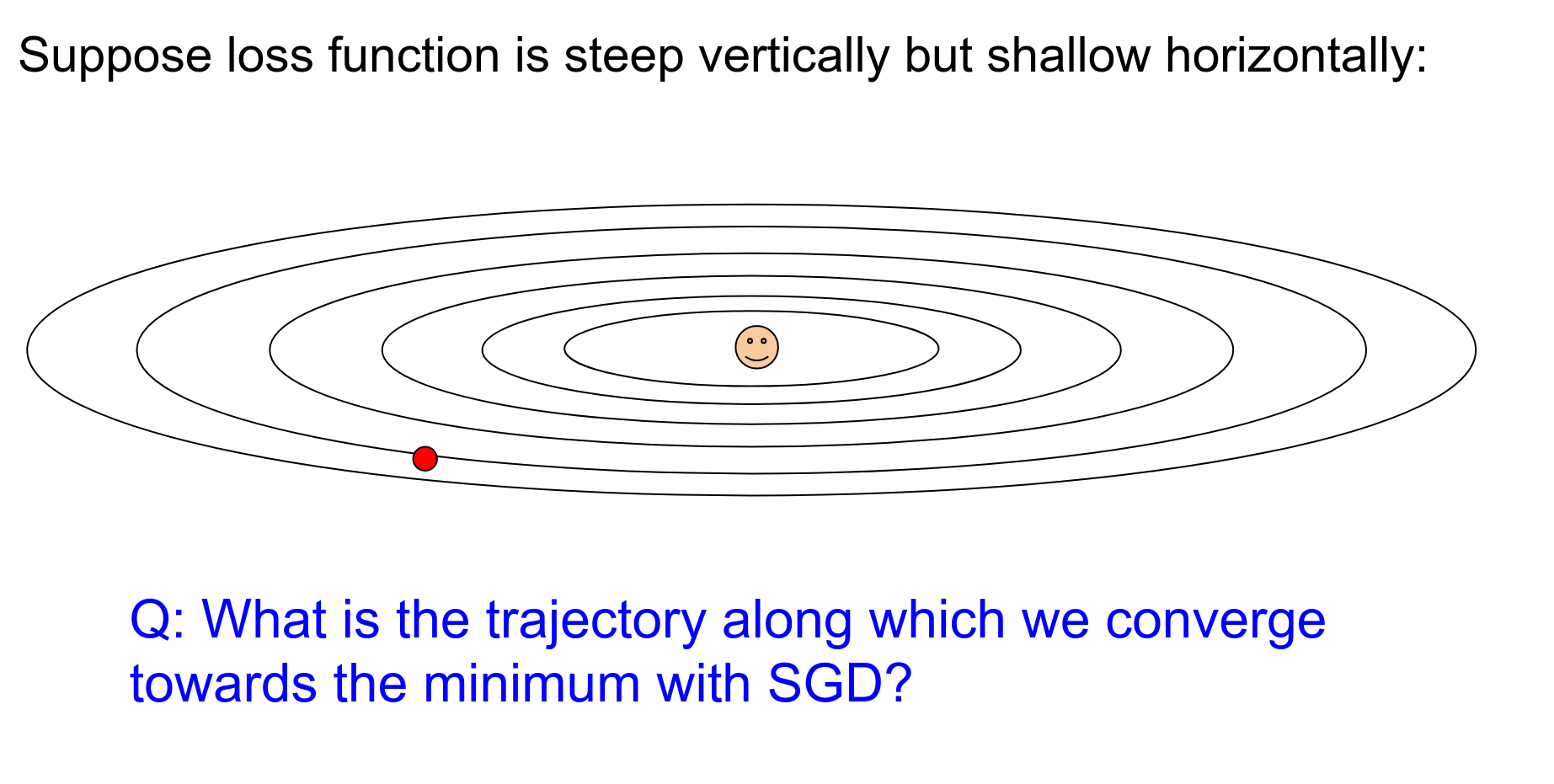
There is a big arrow pointing up and a small one pointing right.
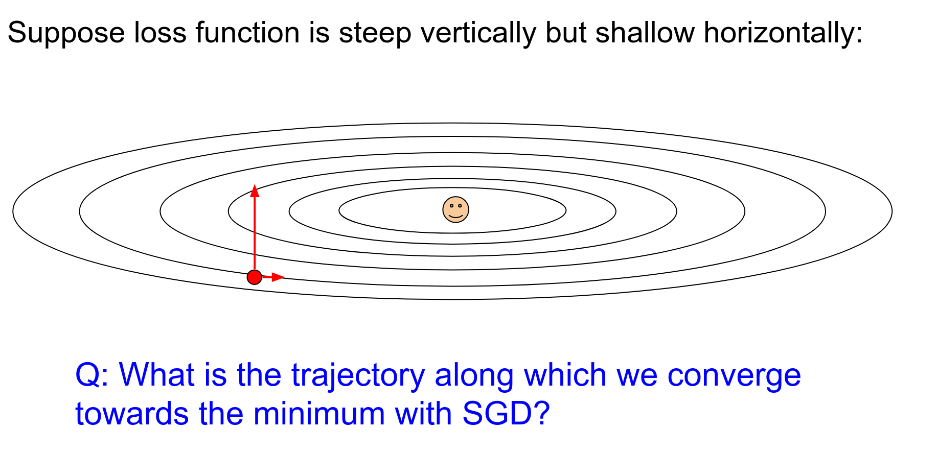
You are going way too fast in one direction and very slow in the other. This results in jitter.
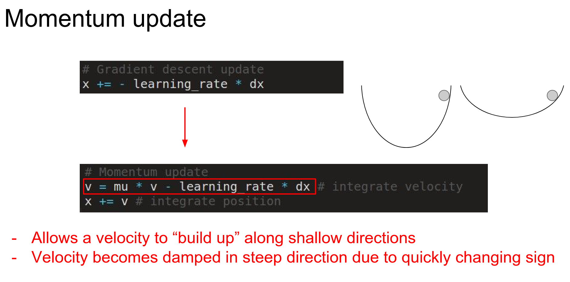
Momentum
\(mu\) is a hyperparameter between 0 and 1.
To solve this problem, we can use momentum.
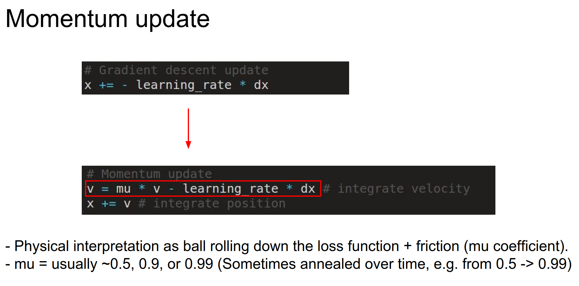
We don't use the learning rate directly; instead, we use velocity to make an update.
Think of a ball rolling around and slowing down over time:
- Gradient is force.
- \(mu * v\) is friction.
- \(v\) - velocity is initialized with 0.
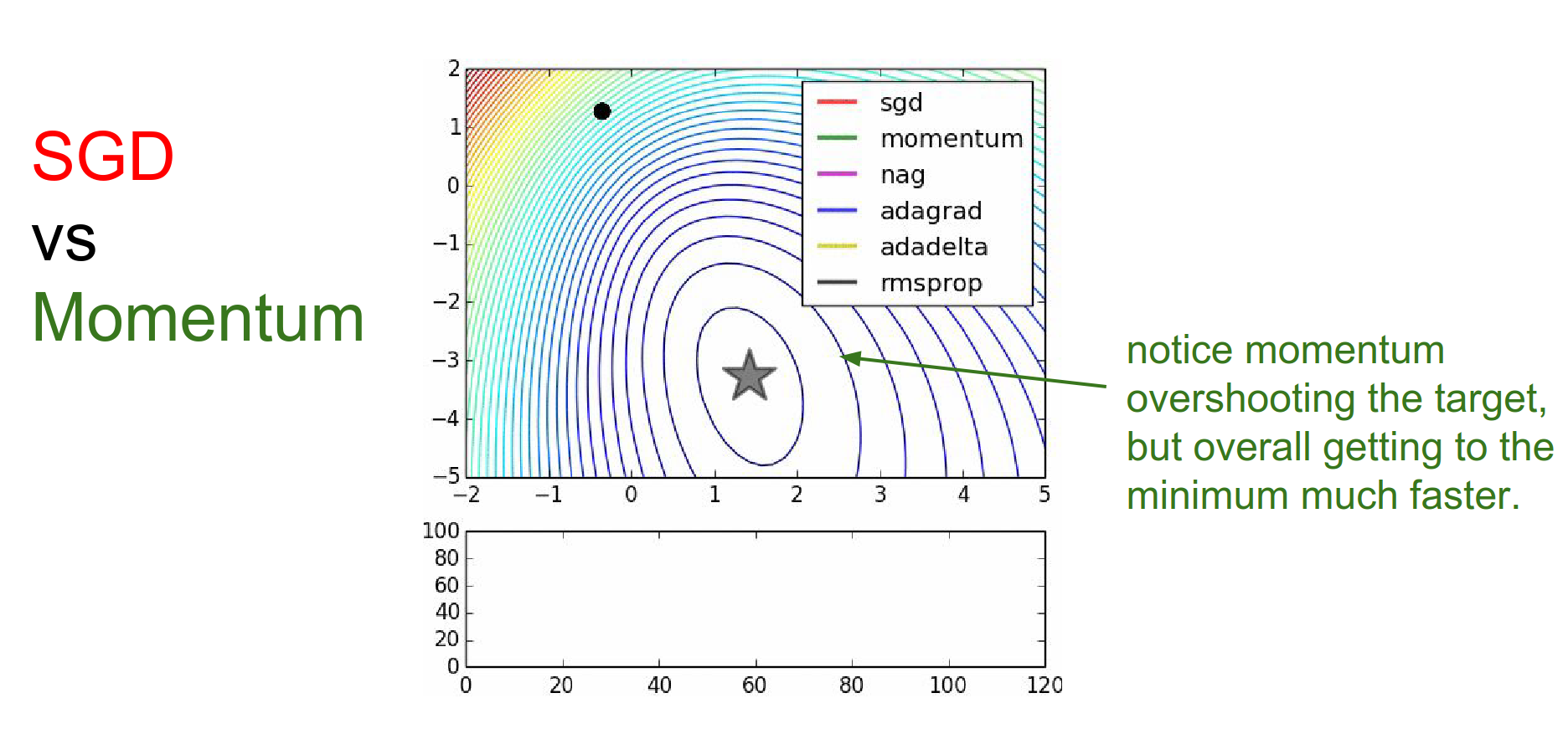
SGD is slower than momentum, as expected. Momentum overshoots the target because it builds up velocity.
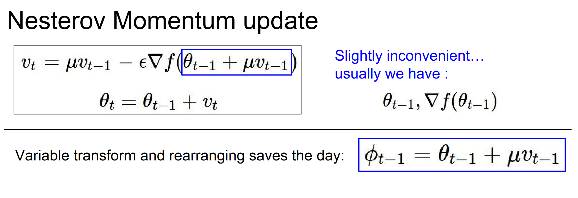
Nesterov Momentum
A variation of Momentum Update.
Momentum and gradient step together? We evaluate the gradient at the end of the momentum step.
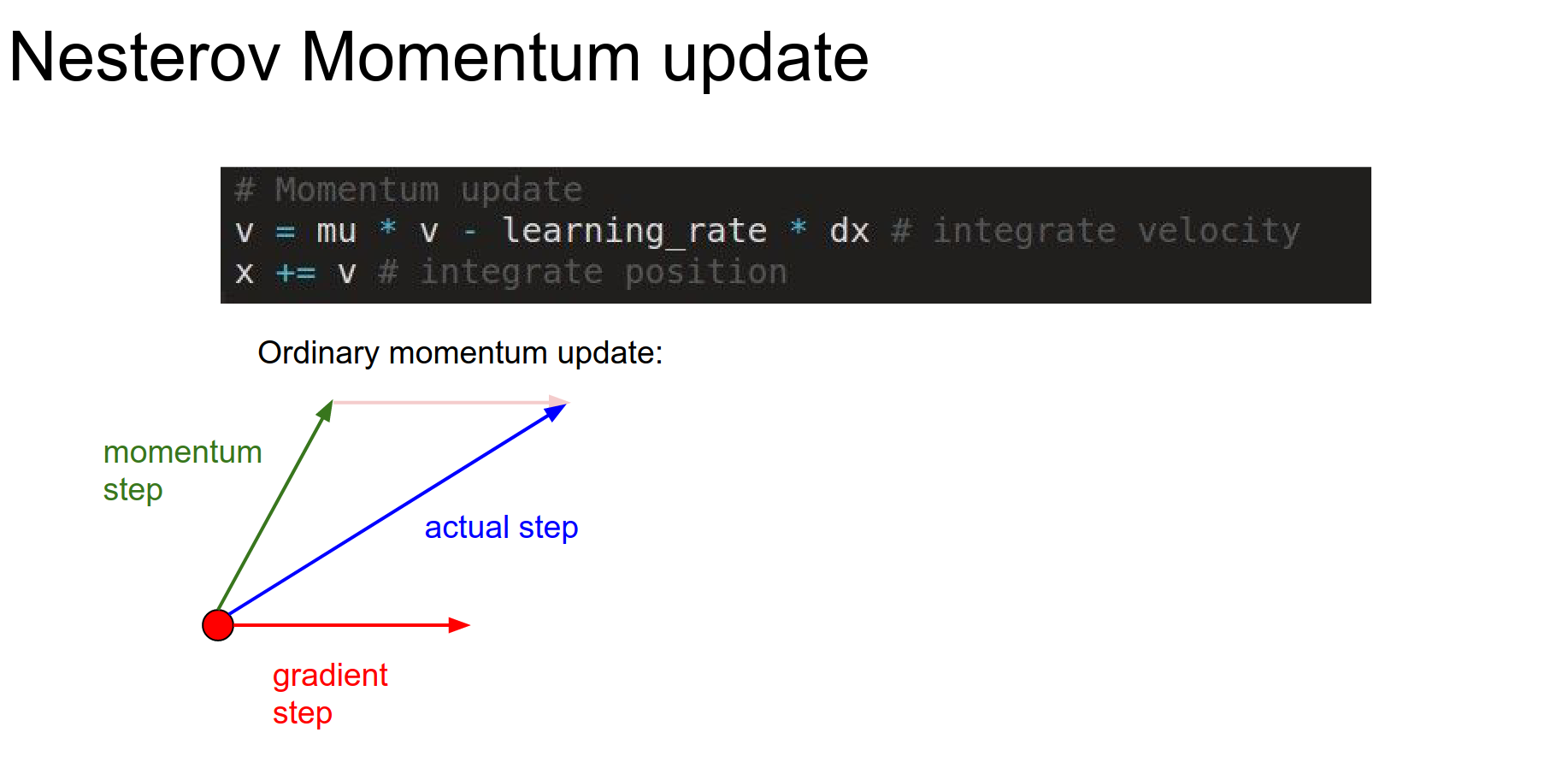
It involves a one-step look-ahead. Evaluate the gradient at the look-ahead step.
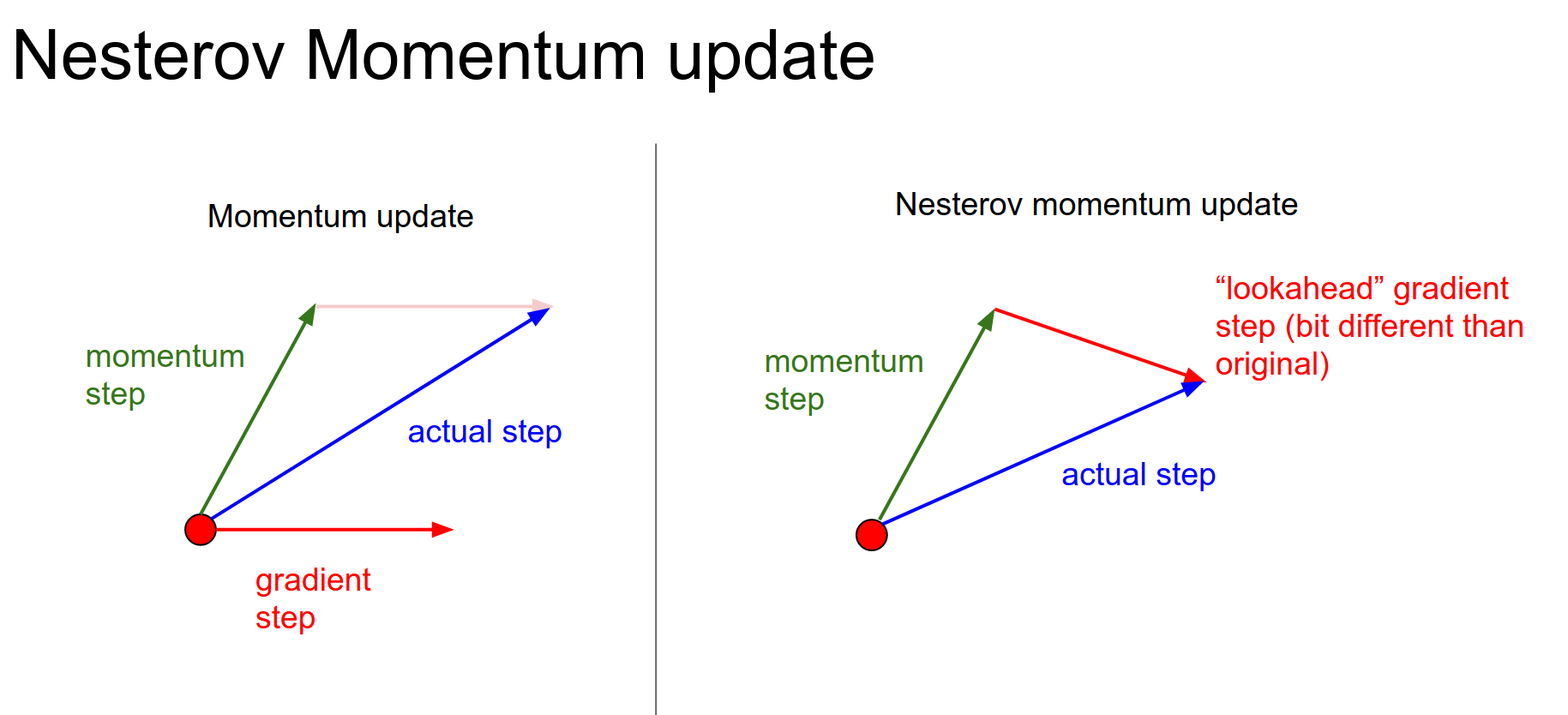
In theory and in practice, it almost always works better than standard momentum.
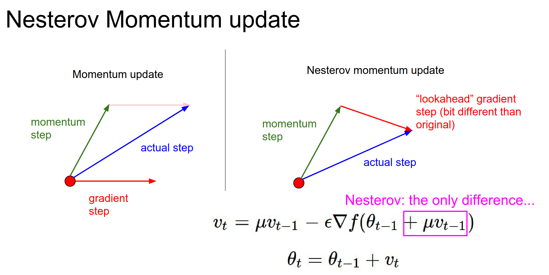
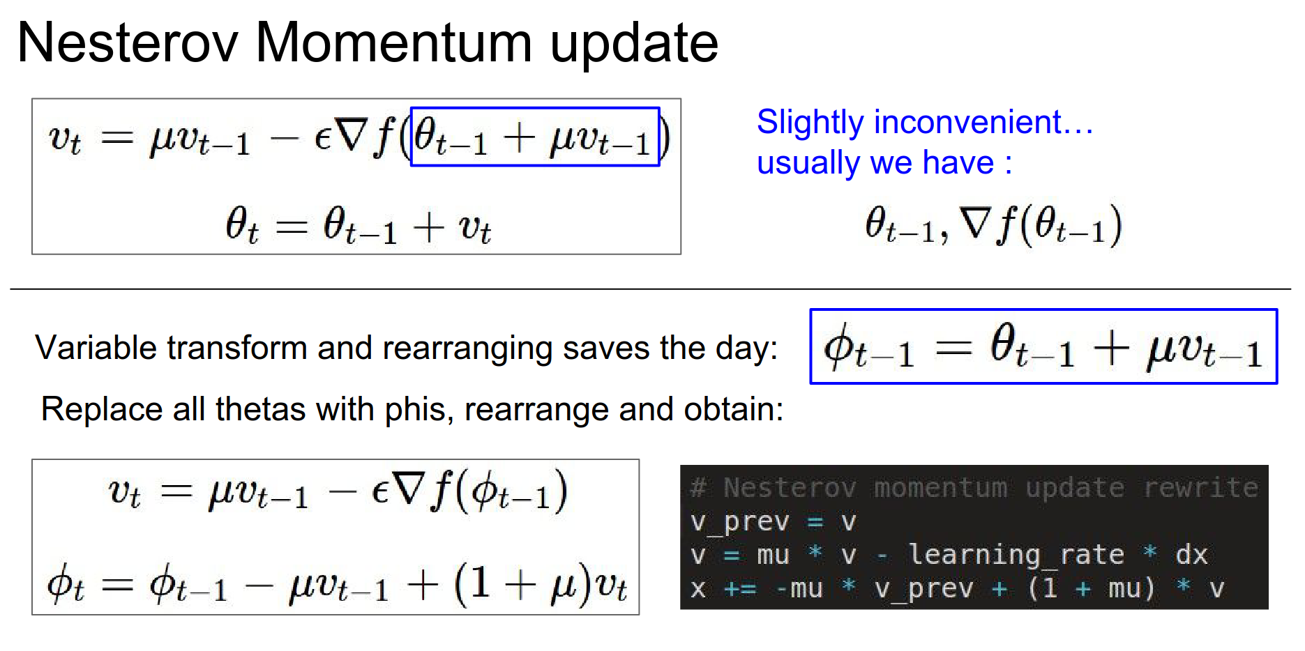
This is a bit ugly and doesn't fit well in a single API. Normally, we do a forward pass and a backward pass, so we usually have a parameter vector and gradient at that point.
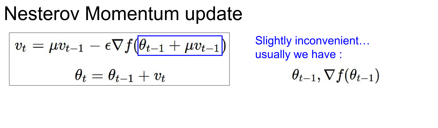
You can perform a variable transform.
You can check the notes for more details.
NAG stands for Nesterov Accelerated Gradient in the graph:
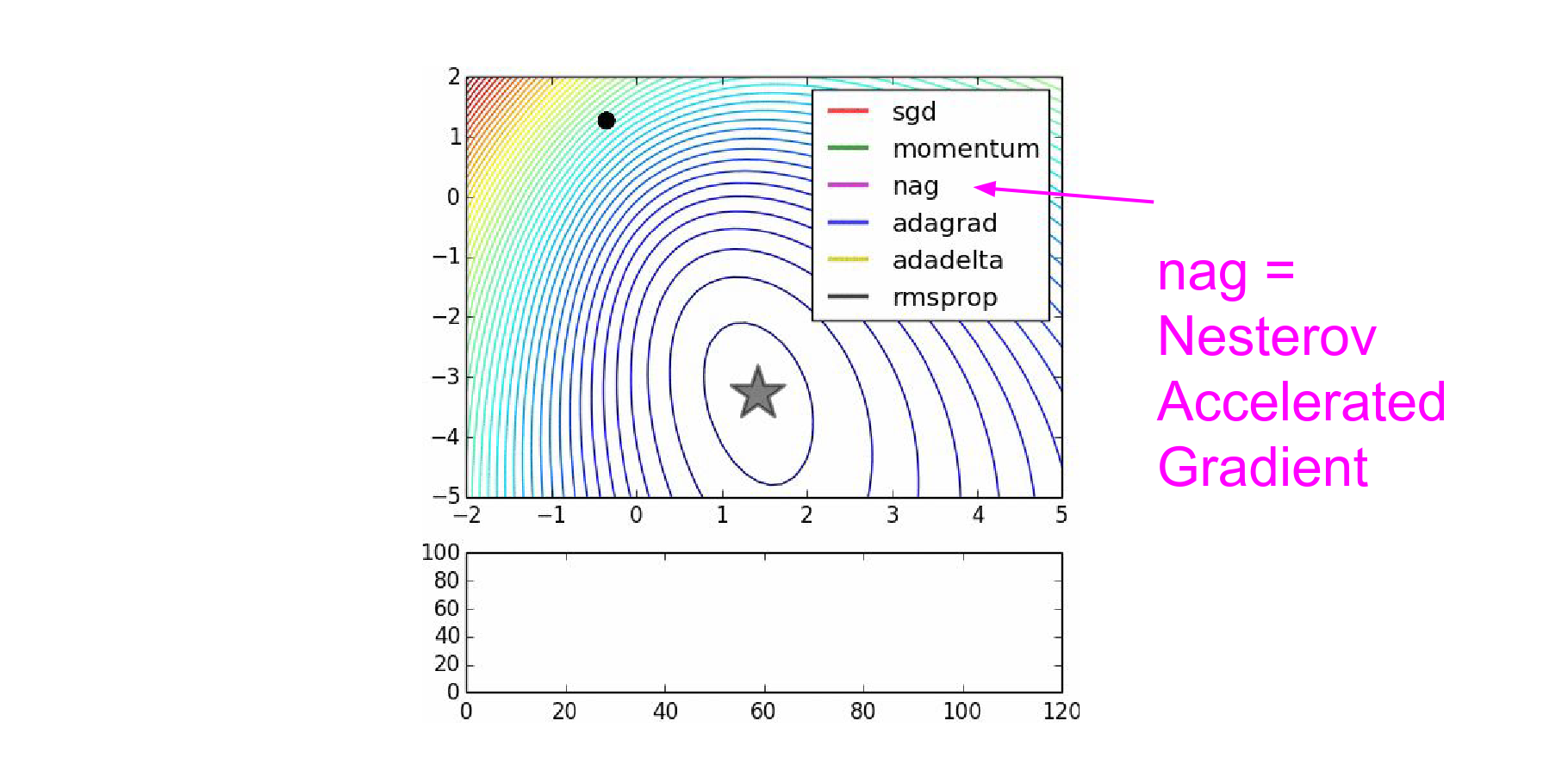
NAG curls around much more quickly than SGD with Momentum. 🍓
Local Minima
As you scale up Neural Networks, the local minima issue goes away; the best and worst local minima get really close.
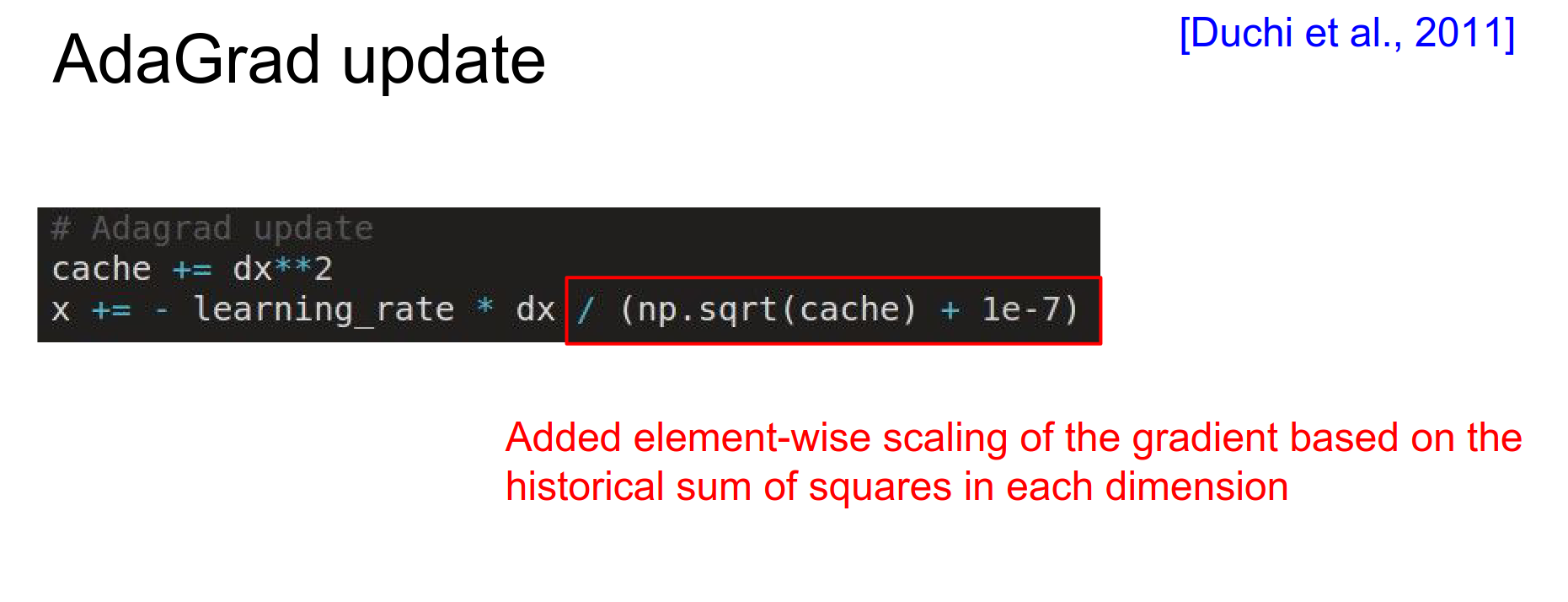
AdaGrad
Is it a scale on SGD?
It is very common in practice. Originally developed in convex optimization literature, it was ported to Neural Networks.
We build a cache which is the sum of squared gradients, a giant vector of the same size as the parameter vector.
Un-centered Second Moment? This is called a per-parameter adaptive learning rate method. Every single dimension of the parameter space now has its own learning rate that is scaled dynamically based on the gradients we are seeing.
What happens with AdaGrad when updating?
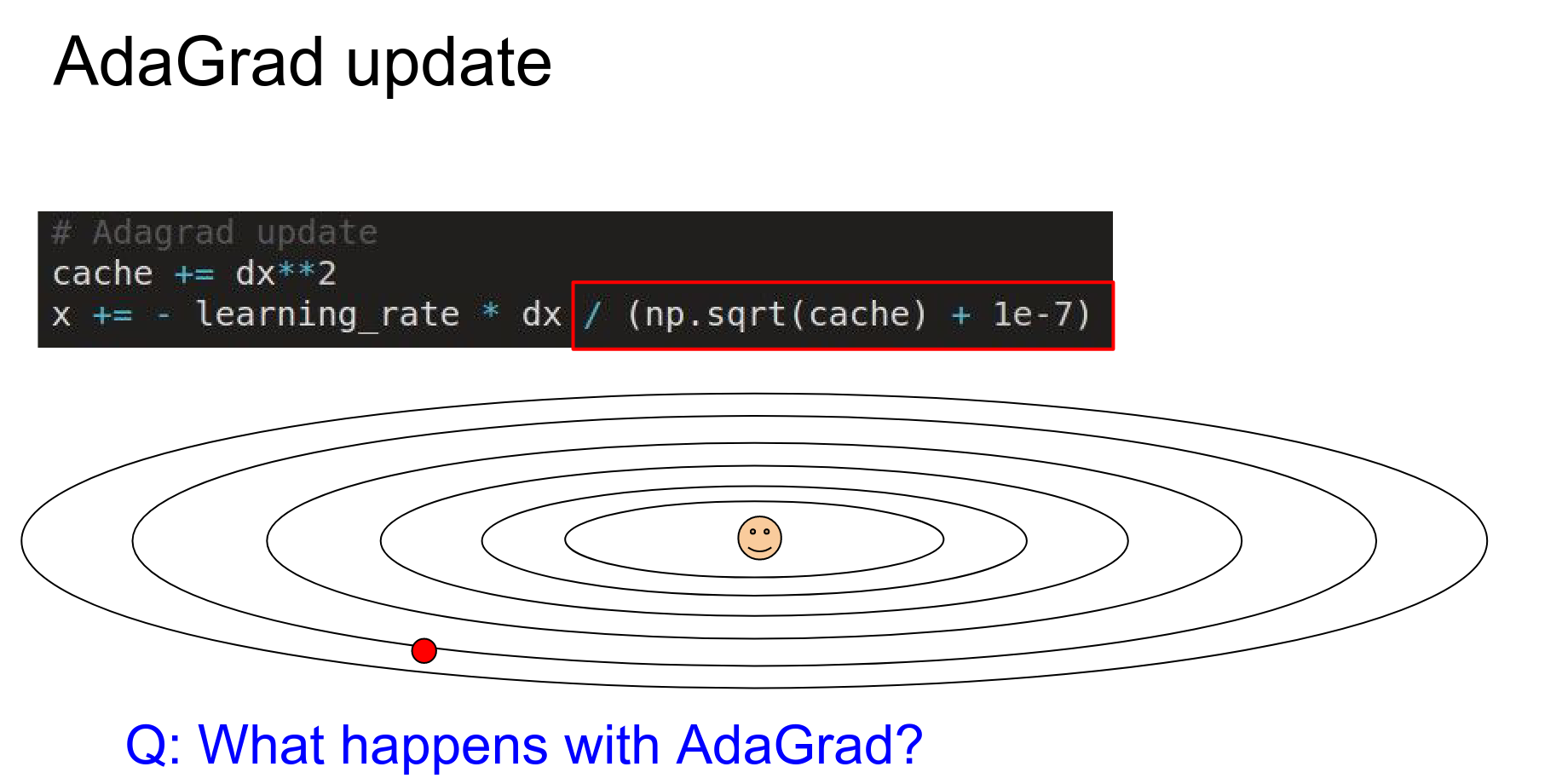
We have a large gradient vertically. That large gradient (fast changes) will be added to the cache, and then we end up dividing by larger and larger numbers, so we'll get smaller and smaller updates in the vertical step.
Since we're seeing lots of large gradients vertically, this will decay the learning rate, and we'll make smaller and smaller steps in the vertical direction.
But in the horizontal direction—which is a very shallow direction—we end up with smaller numbers in the denominator. Relative to the Y dimension, we're going to end up making faster progress.
So we have this equalizing effect of accounting for the steepness, and in shallow directions, you can actually have a much larger learning rate compared to the vertical directions.
That's AdaGrad.
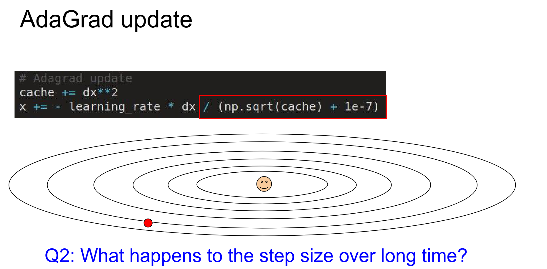
One problem with AdaGrad: it can decay to a halt.
Your cache ends up building up all the time. You add all these positive numbers to your denominator, so your learning rate just decays towards zero, and you end up stopping learning completely.
That's okay in convex problems, perhaps, where you just have a ball and you decay down to the optimum and you're done.
But in a neural network, things are shuffling around and trying to pick your data. It needs continuous energy to fit your data.
You don't want it to just decay to a halt.
1e-7 is there to prevent the division by zero error. It is also a hyperparameter.
rmsprop will forget the gradients from long ago; it is an exponentially weighted sum.
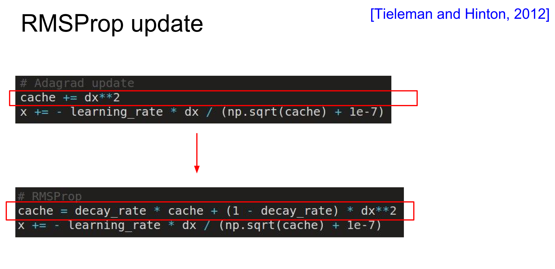
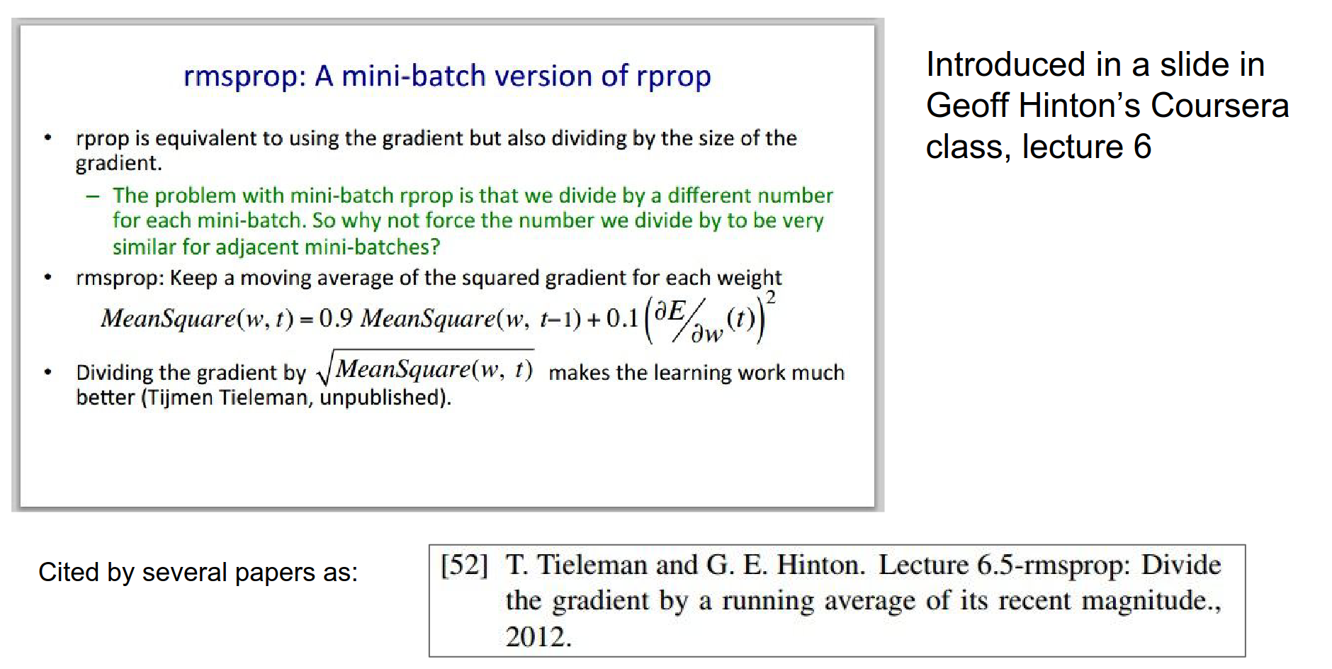
RMSProp
There's a very simple change to AdaGrad that was proposed by Geoff Hinton: rmsprop. 🤭
Instead of keeping just the sum of squares in every single dimension, we make that counter a leaky counter.
We introduce a decay rate hyperparameter, usually set to something like 0.99. You accumulate the sum of squares, but it leaks slowly with this decay rate.
We still maintain this nice equalizing effect of step sizes in steep or shallow directions, but we won't converge completely to zero updates.
It was just a slide in a Coursera course.
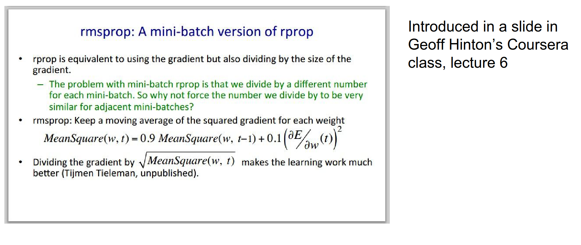
People cited this slide. 😅
Here is the image again. AdaGrad is blue, RMSProp is black.
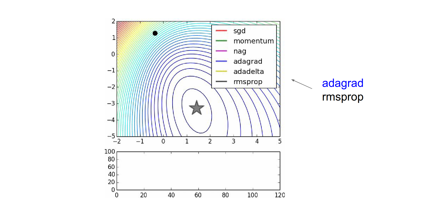
Usually, in practice when training deep neural networks, adagrad stops too early, and rmsprop ends up winning out.
Adam
Combine AdaGrad with Momentum. 🍉
Adam is a recent update that has elements of both.
The Adam optimizer is not necessarily the "best" for all neural networks, but it is a popular and effective choice for many applications. There are several reasons for its popularity:
-
Adaptive learning rate: Adam optimizer adapts the learning rate for each parameter, which helps in faster convergence and better performance. It combines the advantages of two other popular optimization methods, AdaGrad and RMSProp, by using the first moment estimate (mean) and the second moment estimate (variance) of the gradients.
-
Memory efficiency: Unlike other adaptive learning rate methods like AdaGrad and RMSProp, Adam only requires the storage of two additional moments (mean and variance) per parameter, making it more memory-efficient.
-
Easy to implement: Adam is relatively easy to implement, as it only requires the computation of the mean and variance of the gradients, which can be done efficiently using moving averages.
-
Robust performance: Adam has been shown to perform well on various optimization tasks, including deep neural networks, making it a popular choice among practitioners.
However, it is essential to note that the choice of optimizer depends on the specific problem and the nature of the data. It is always recommended to experiment with different optimizers and tune their hyperparameters to find the best fit for a given task.
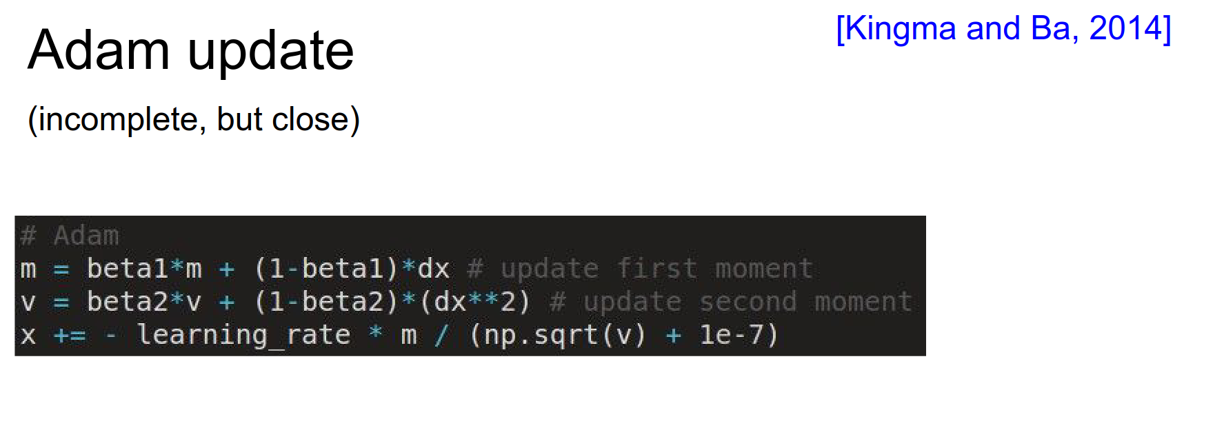
It's kind of like both together.
In \(m\), it sums up the raw gradients, keeping the exponential sum.
In \(v\), it keeps track of the second moment of the gradient and its exponential sum.
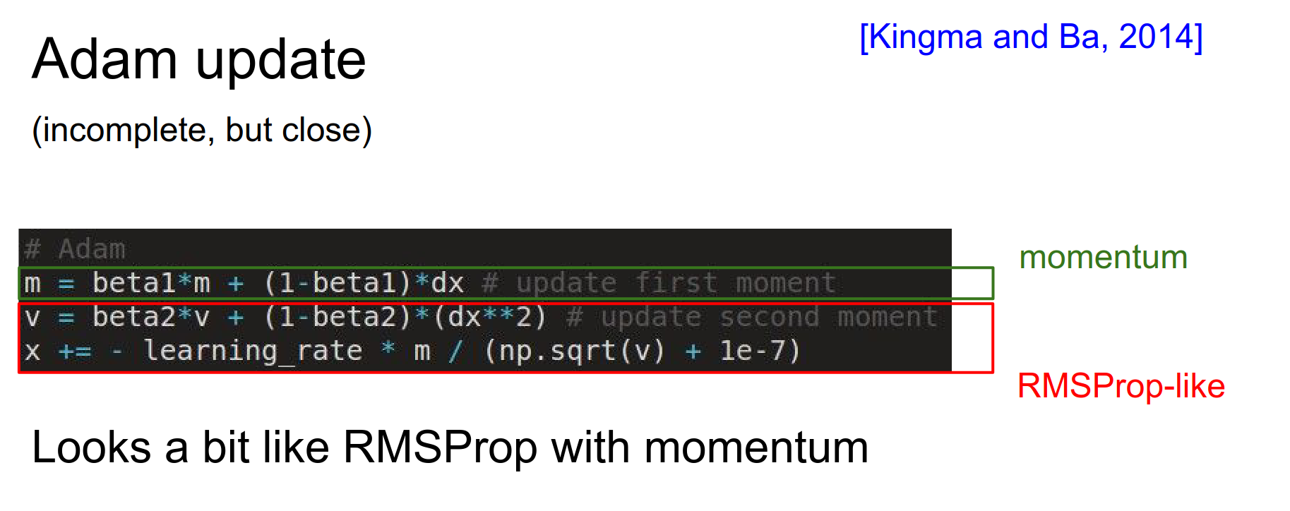
If we compare rmsprop with Momentum and Adam:
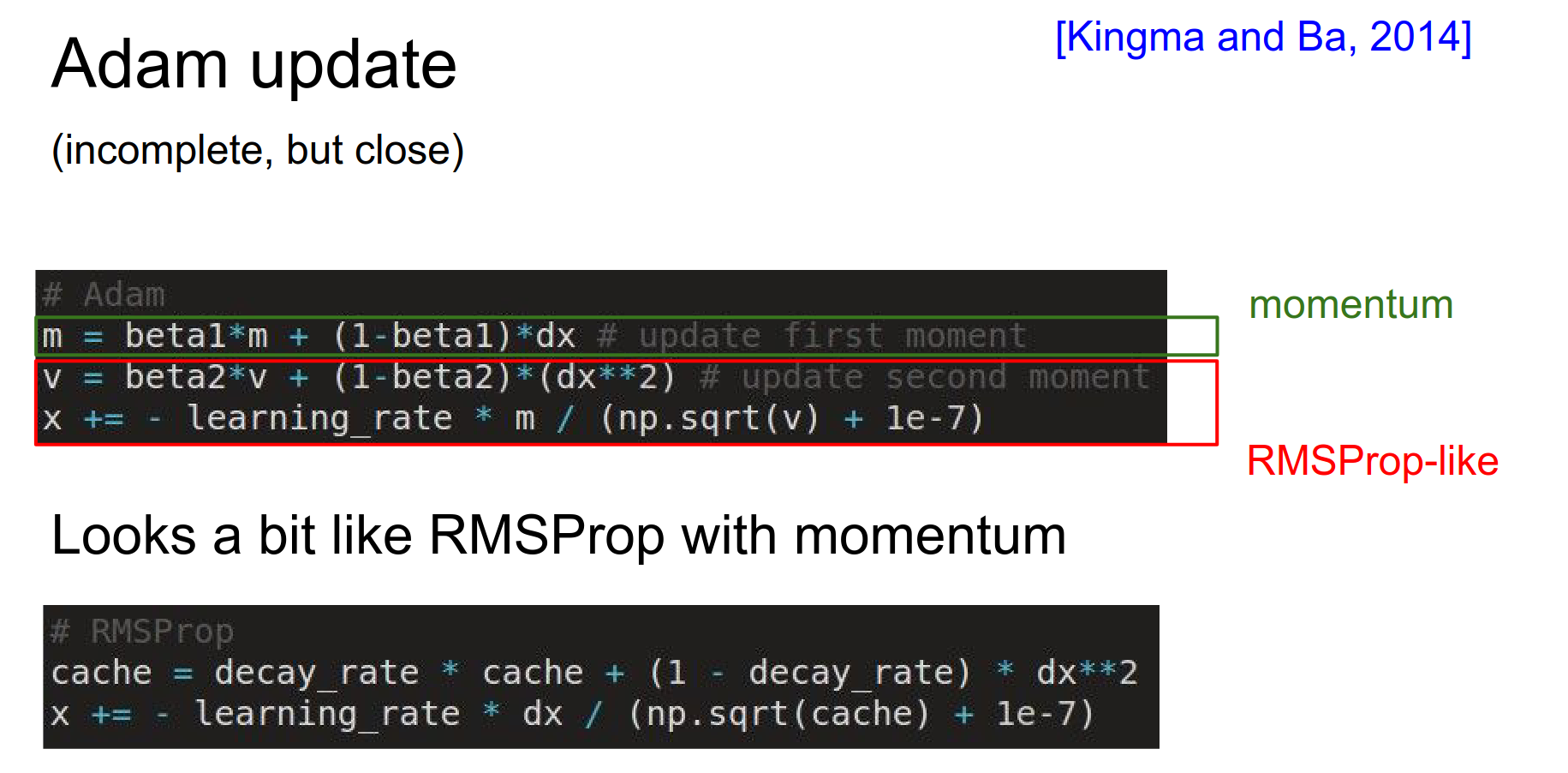
Beta1 and Beta2 are hyperparameters. Usually, \(beta1 = 0.9\) and \(beta2 = 0.995\).
We replace the \(dx\) (in the second equation) in RMSProp with \(m\), which is the running counter of \(dx\).
At any time, you will have noisy gradients. Instead of using those noisy gradients, you use a weighted (decaying) sum of previous gradients, which stabilizes the gradient direction.
The fully complete version is shown below:
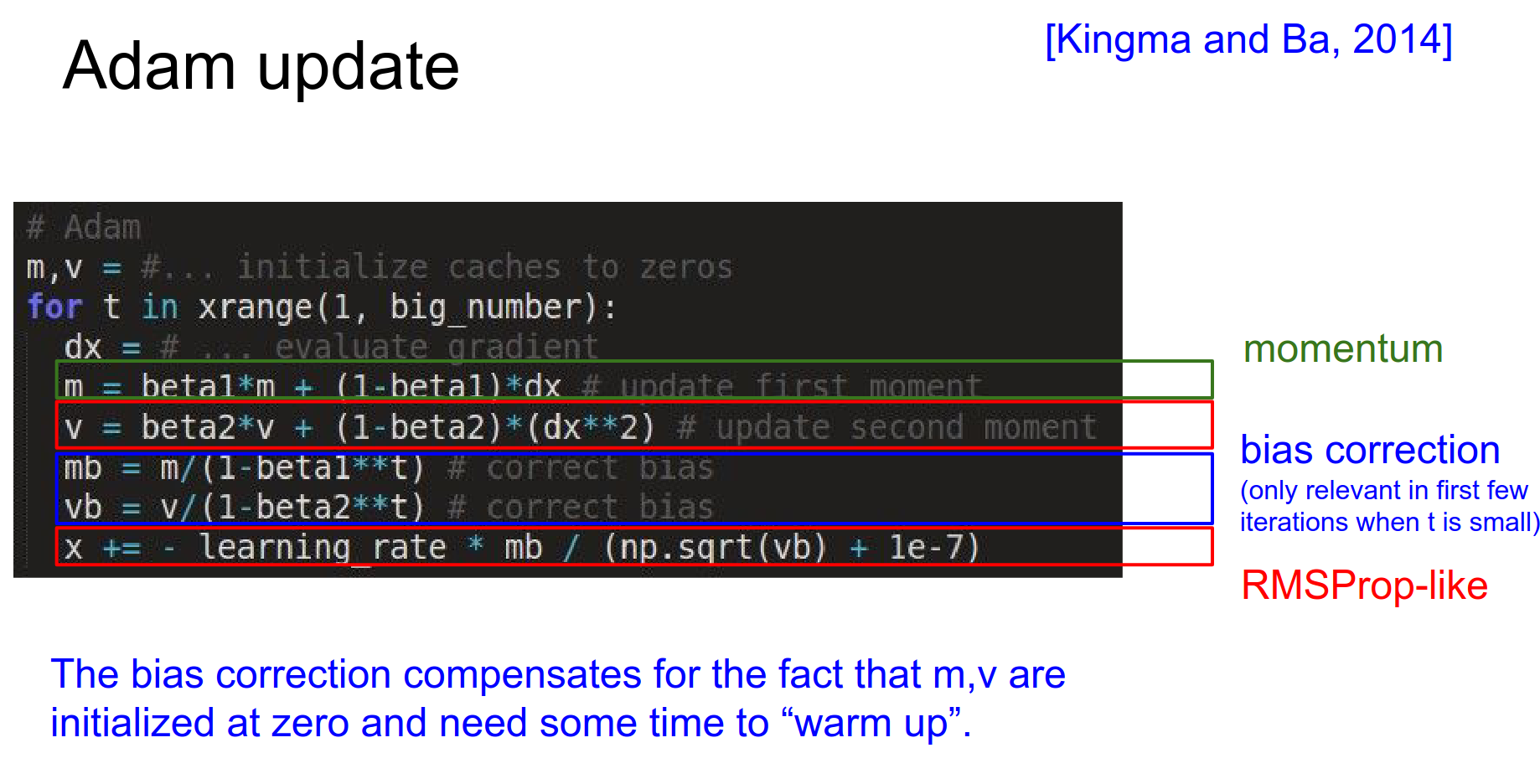
There is also bias correction, which depends on the time step \(t\). Bias correction is only important as Adam is warming up.
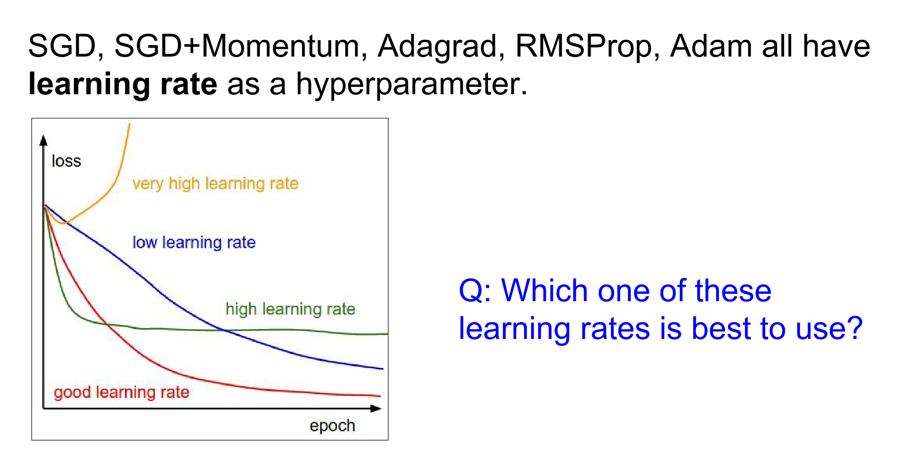
It depends.
You should start with a high learning rate. It optimizes faster. At some point, you will be too stochastic and cannot converge to your minima nicely because you have too much energy in your system and cannot settle down into the nice parts of your loss function.
Decay your learning rate, and you can ride this wagon of decreasing learning rates to do best in all of them.
Epoch
1 Epoch means you have seen all of the training data once.
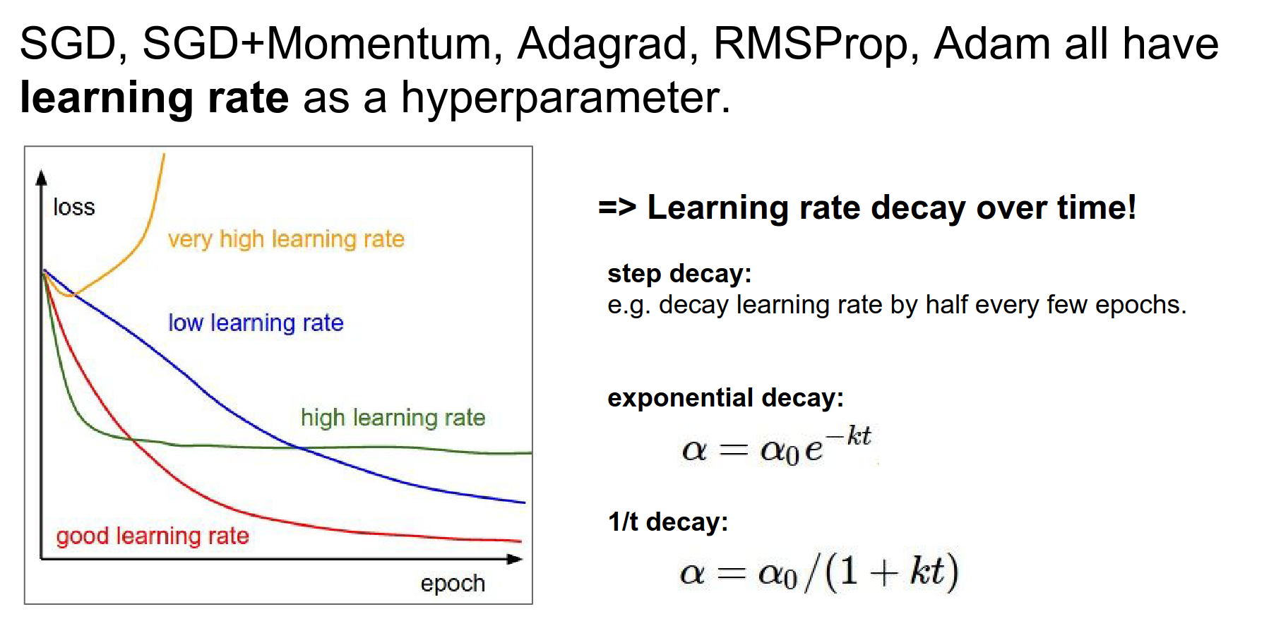
Learning Rate Decays
Step - Exponential - 1/t
These learning rate decays are solid for SGD and Momentum SGD. Adam and AdaGrad are less dependent on them.
Andrej uses Adam for everything now. 🥳
These are all first-order methods because they only use the gradient information of your loss function. When you evaluate the gradient, you know the slope in every single direction.
Second Order Methods
These provide a better approximation to your loss function. They do not only approximate with the hyperplane (which way we are sloping) but also approximate it with the Hessian, telling you how your surface is curving.
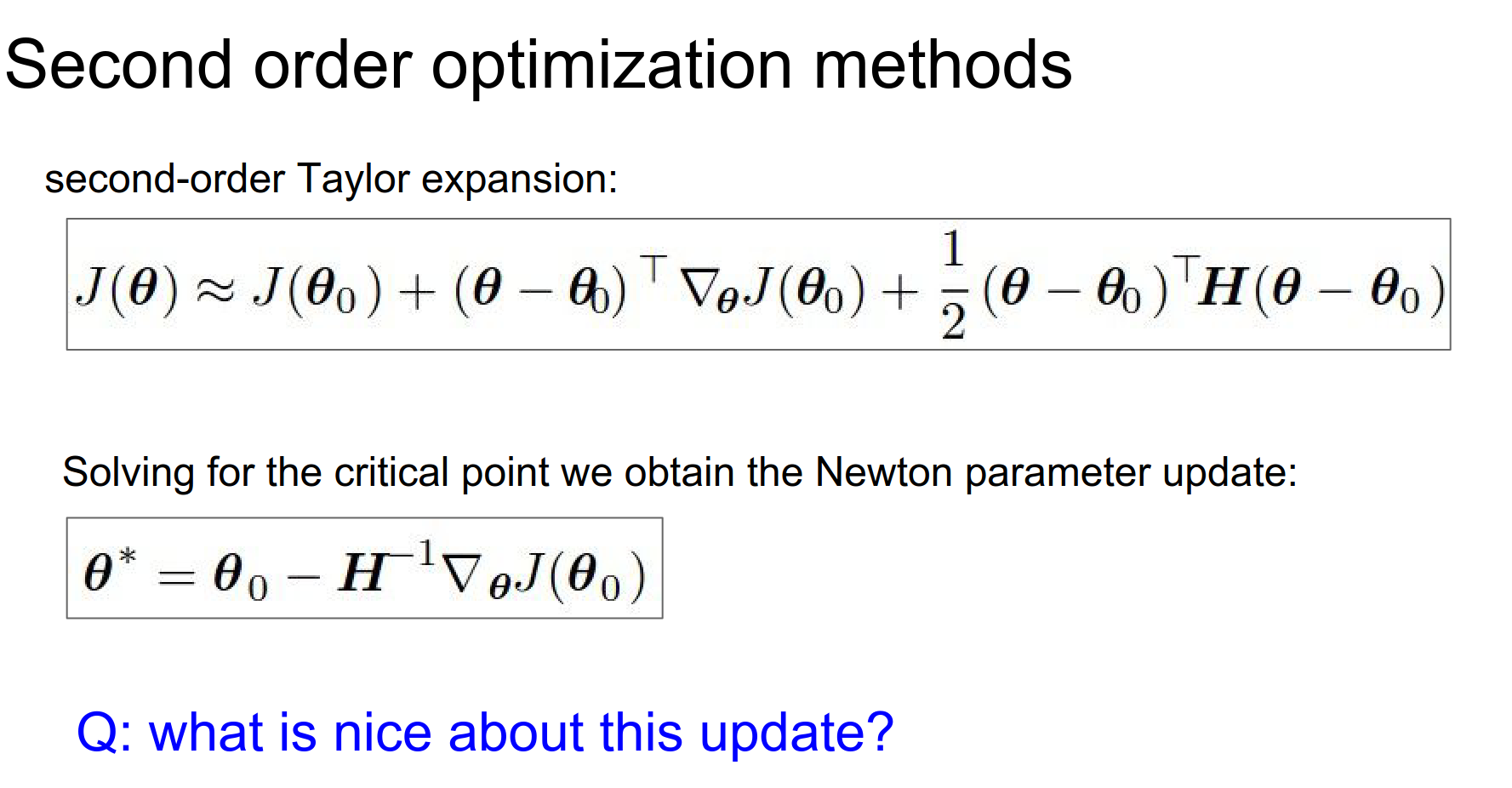
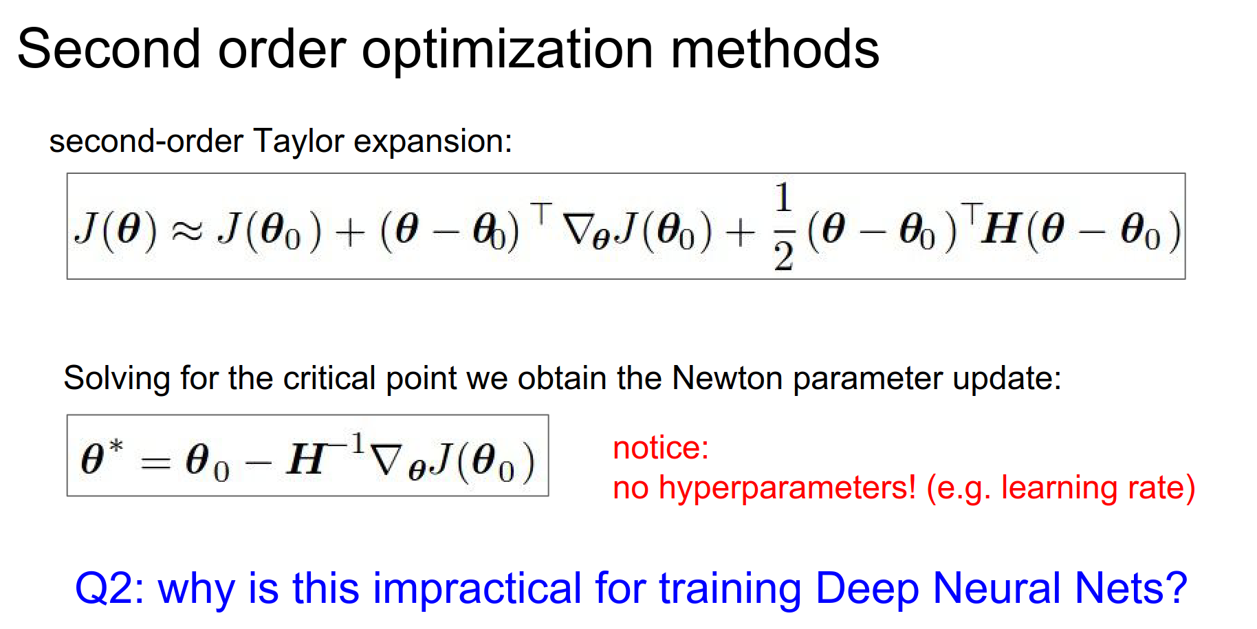
- Faster convergence
- Fewer Hyperparameters - No need for a learning rate.
- Your Hessian will be gigantic:
- If you have a 100 million parameter network, your Hessian will be
100mil x 100mil, and you want to invert it.
So, this is not a good idea in Neural Networks.
You can get around inverting the Hessian using BGFS and L-BFGS.
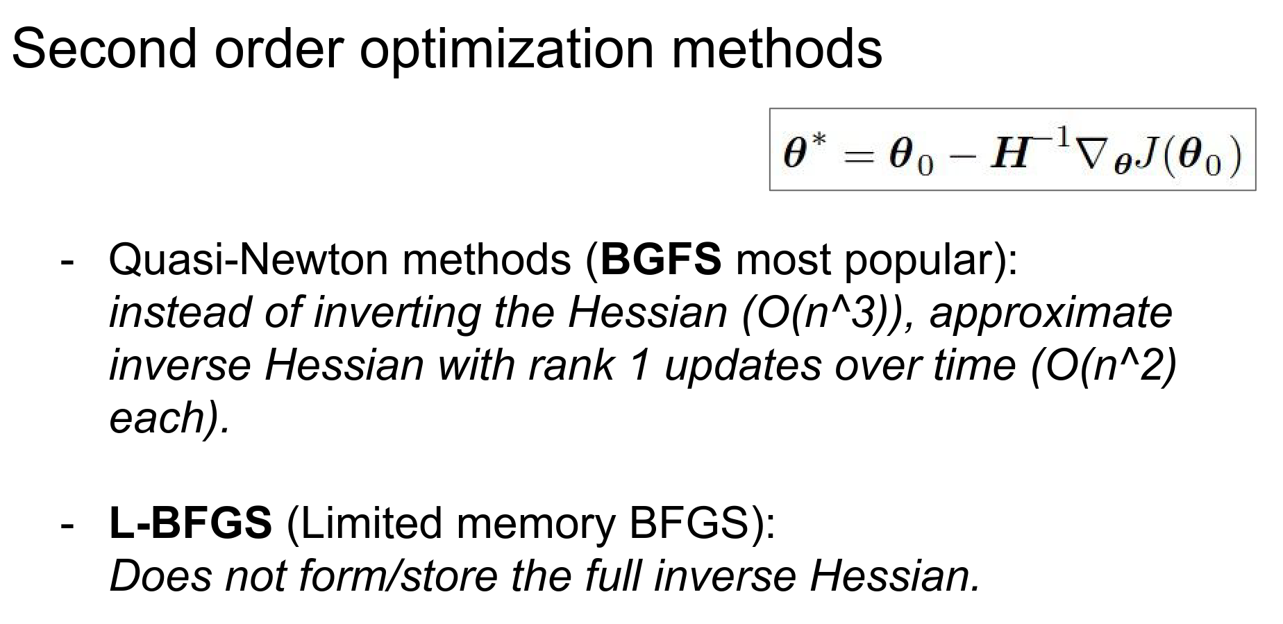
These are used in practice.
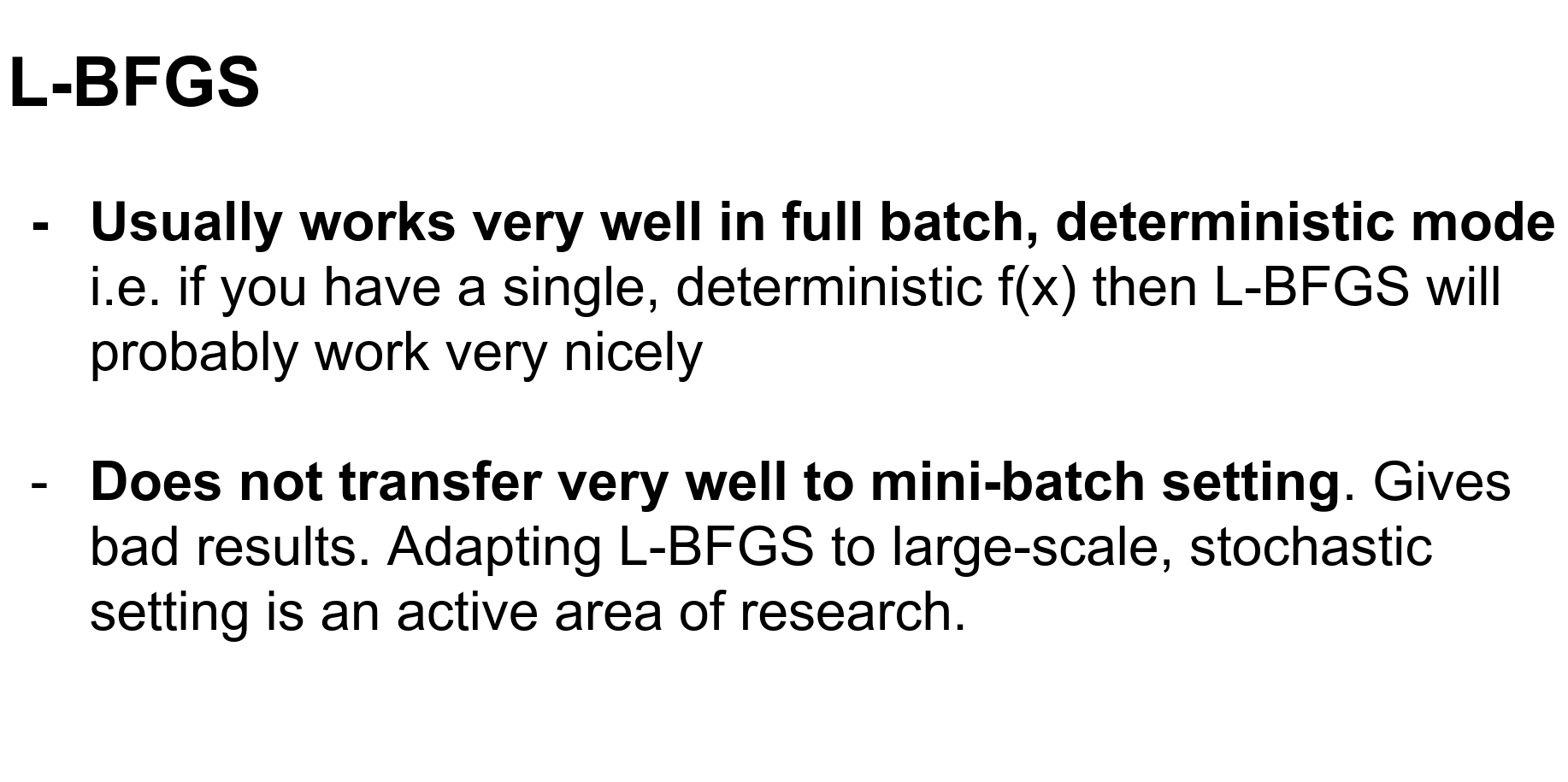
L-BFGS works really well on \(f(X)\) functions. In mini-batches, it doesn't work well.
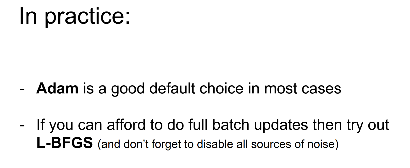
Adam is the default. If you have a small dataset, you can look up L-BFGS.
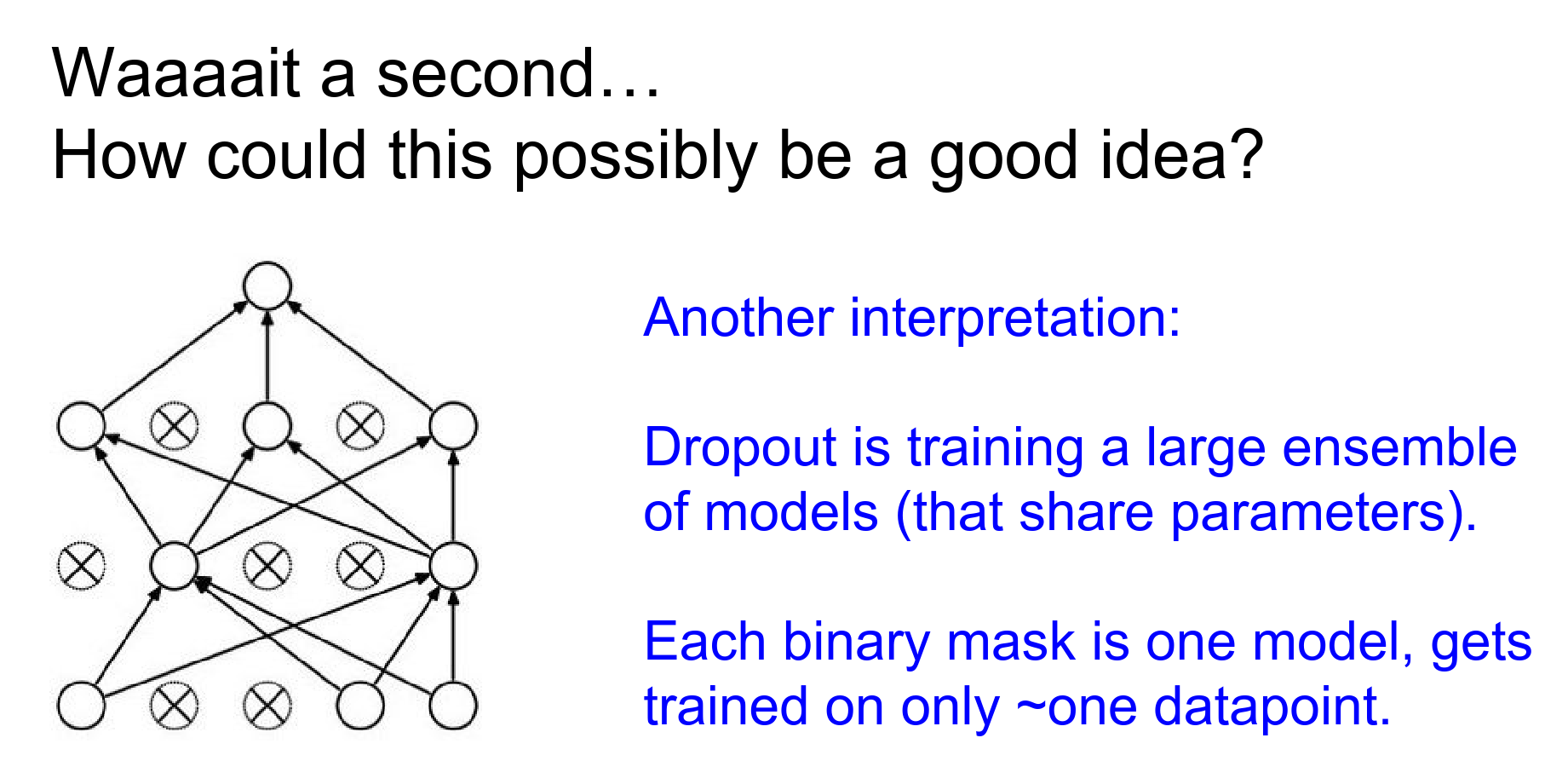
What does that mean?
Multiple models, average the results. You have to train all of these models, so that is not ideal.
You save a checkpoint when you are training.
Model Ensembles
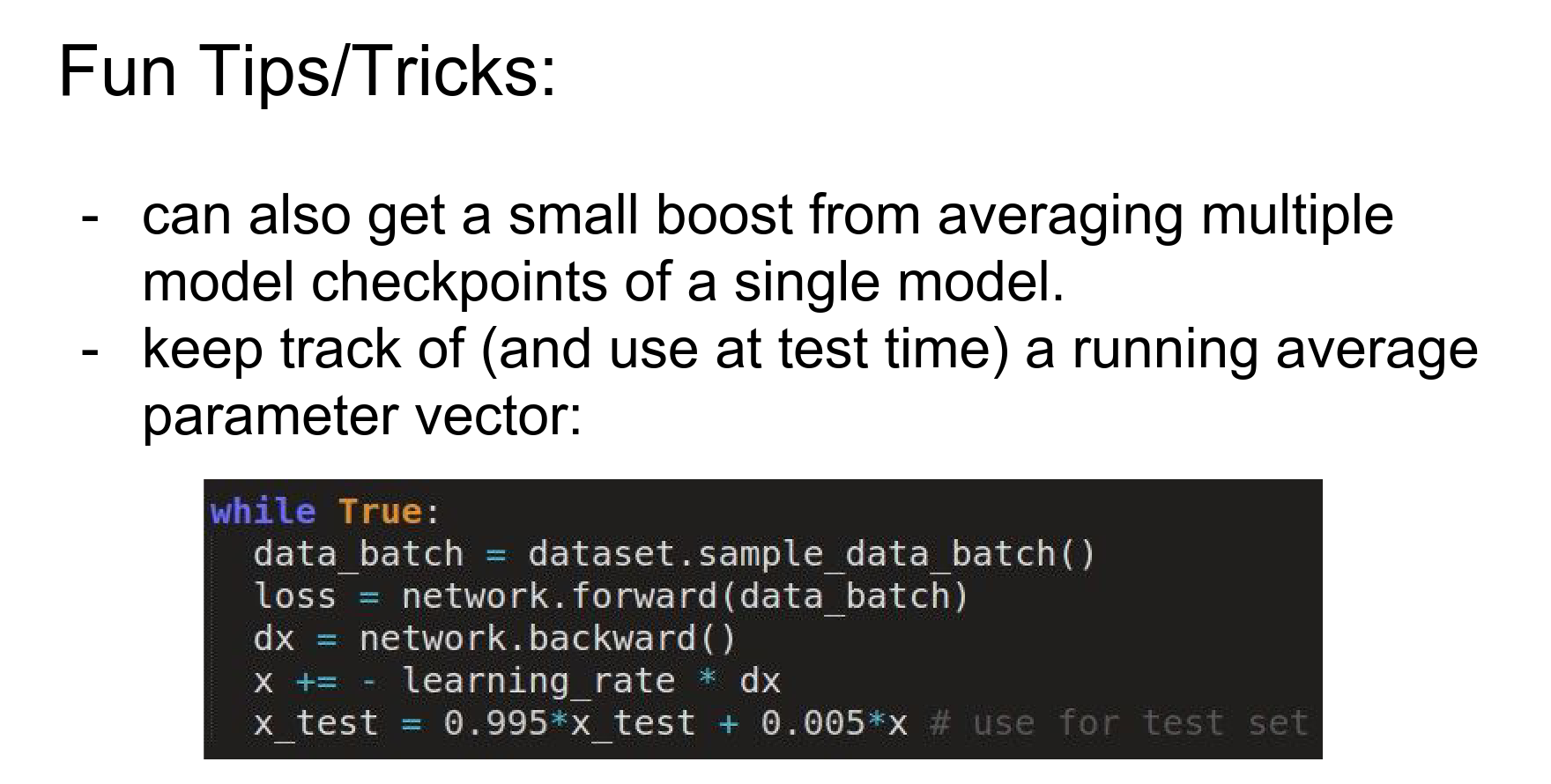
x_test is a running sum, exponentially decaying. This x_test works better on validation data.
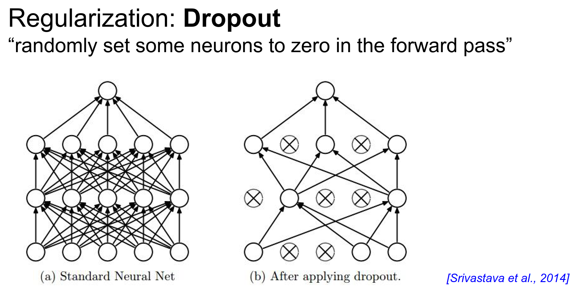
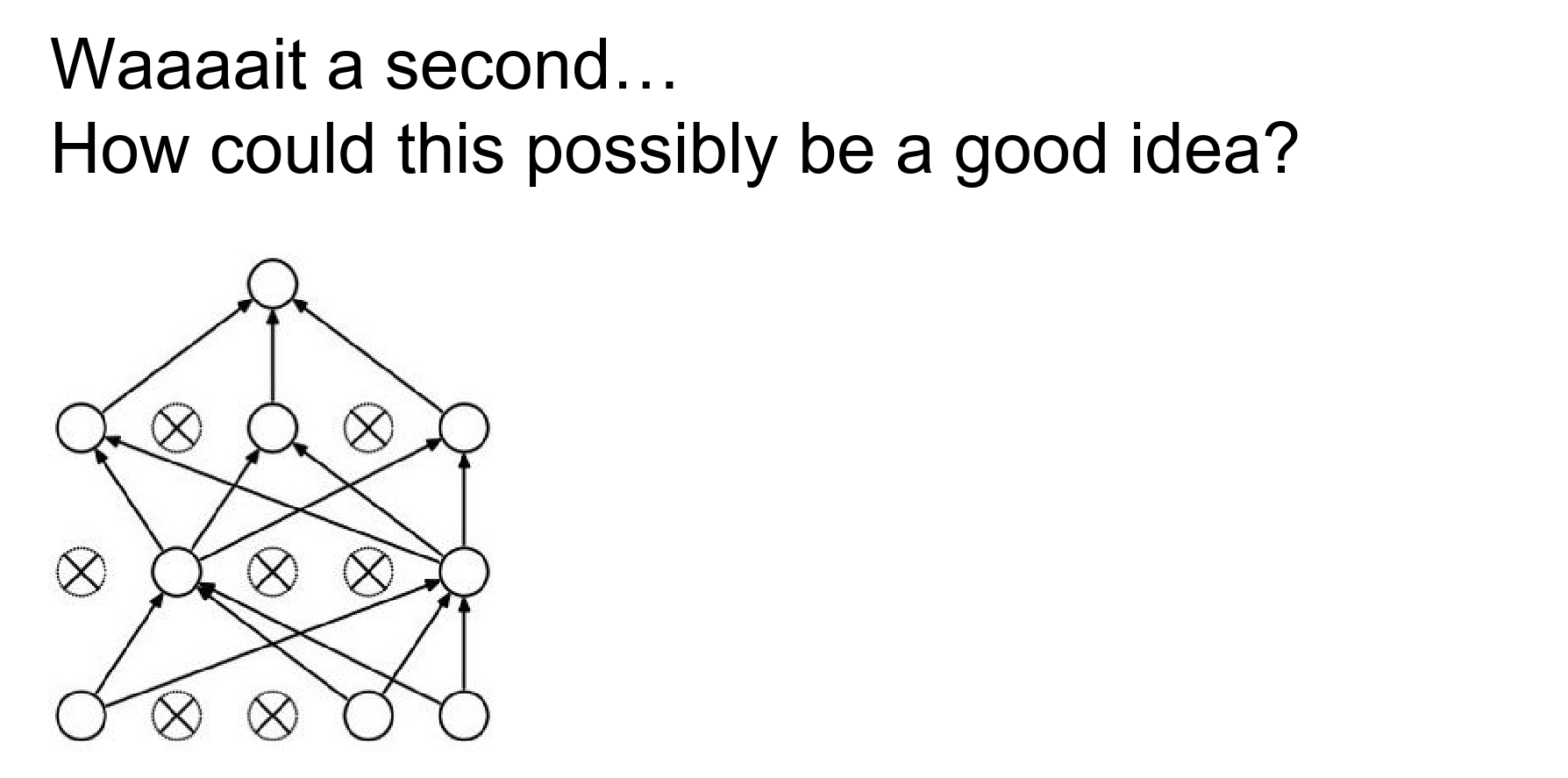
Dropout
A very important technique.
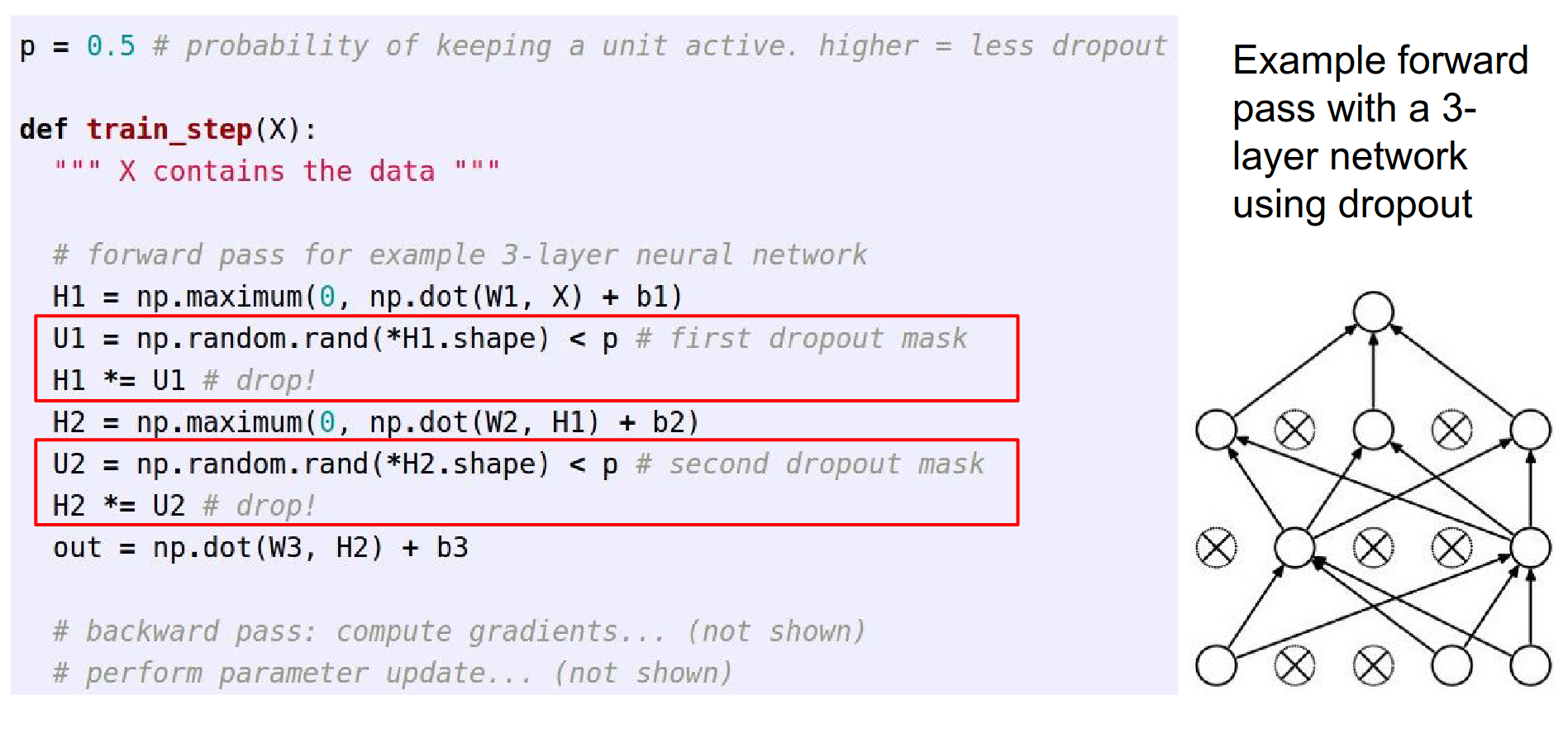
As you are doing a forward pass, you set some neurons randomly to zero.
\(U1\) is zeros and ones, a binary mask. We apply this mask to hidden layer 1 \(H1\) (effectively dropping half of them).
We also do this for the second hidden layer. Do not forget we need to consider this in the backward pass too.
Motivation
Maybe it will prevent overfitting? All features can have the same strength.
It forces all the neurons to be useful.
Feature Co-adaptation
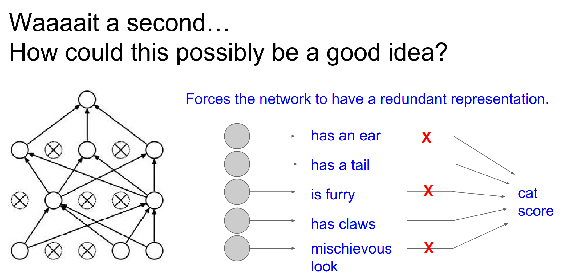
You cannot rely on a single feature.
A dropped-out neuron will not have connections to the previous layer, as if it were not there.
You are sub-sampling a part of your Neural Network, and you are only training that neural network on that single example that you have at that point in time.
You want to apply stronger dropout where there is a huge number of parameters.
In practice, you do not use dropout at the start of Convolutional Neural Networks; you scale the dropout over time.
Instead of dropping gradients, you can drop weights. That is called DropConnect.
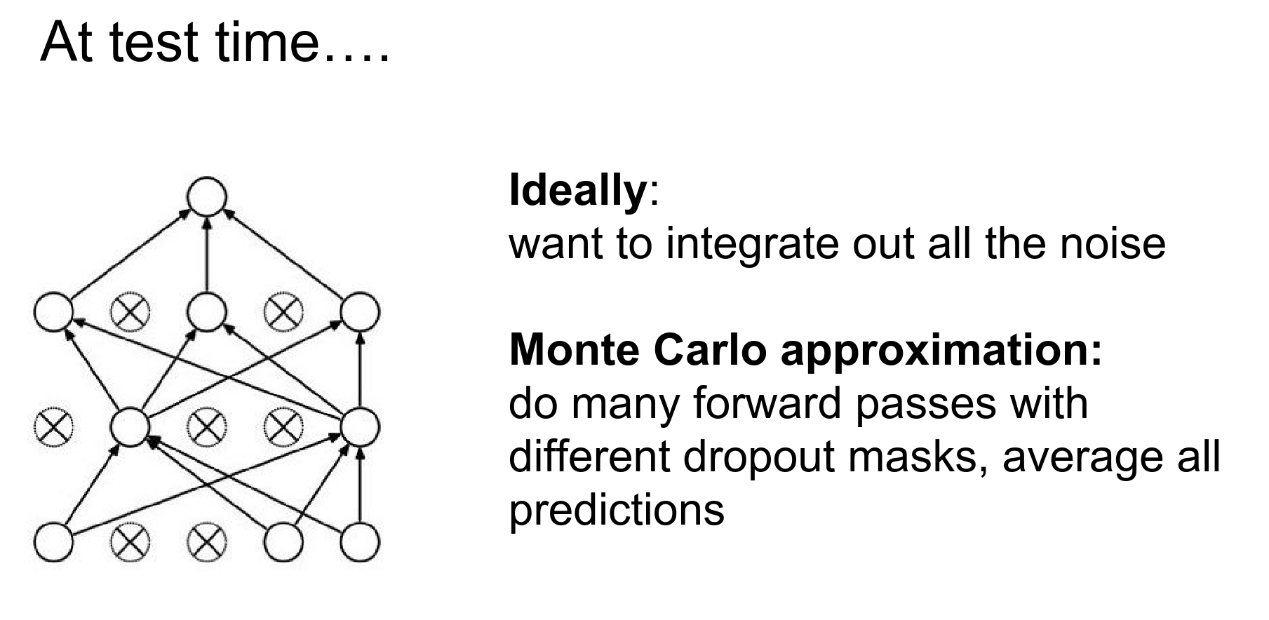
We would like to integrate out all of the noise. You can try all binary masks and average the result, but that is not really efficient.
You can approximate this with Monte Carlo.
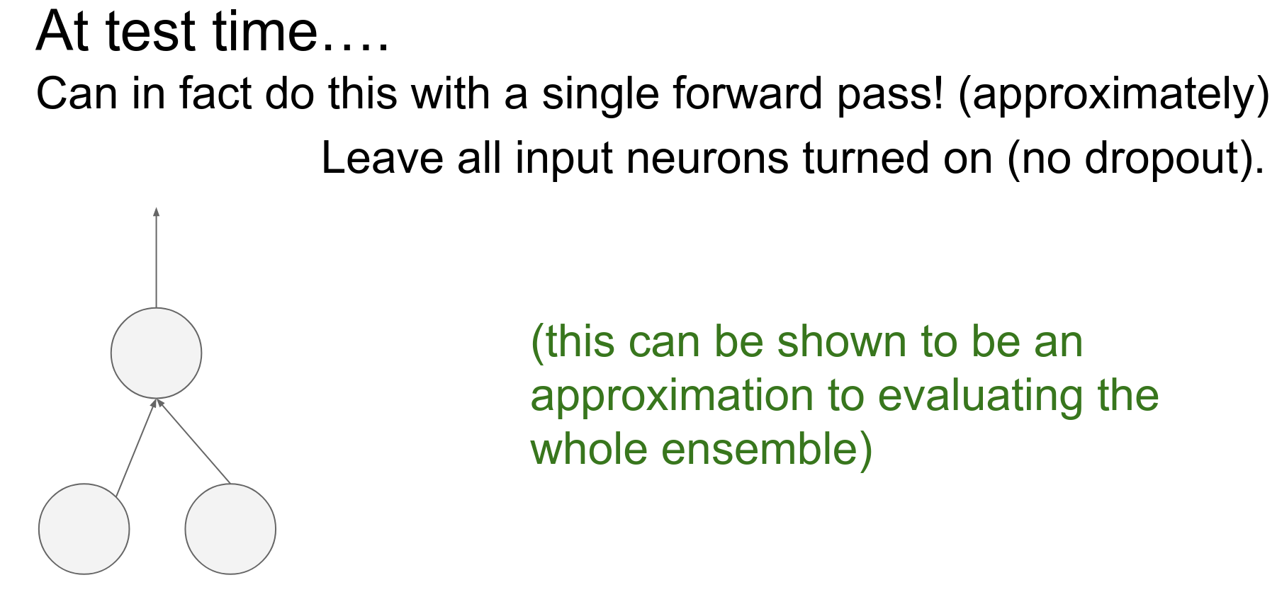
In an ideal world, you do not want to leave any neurons behind.
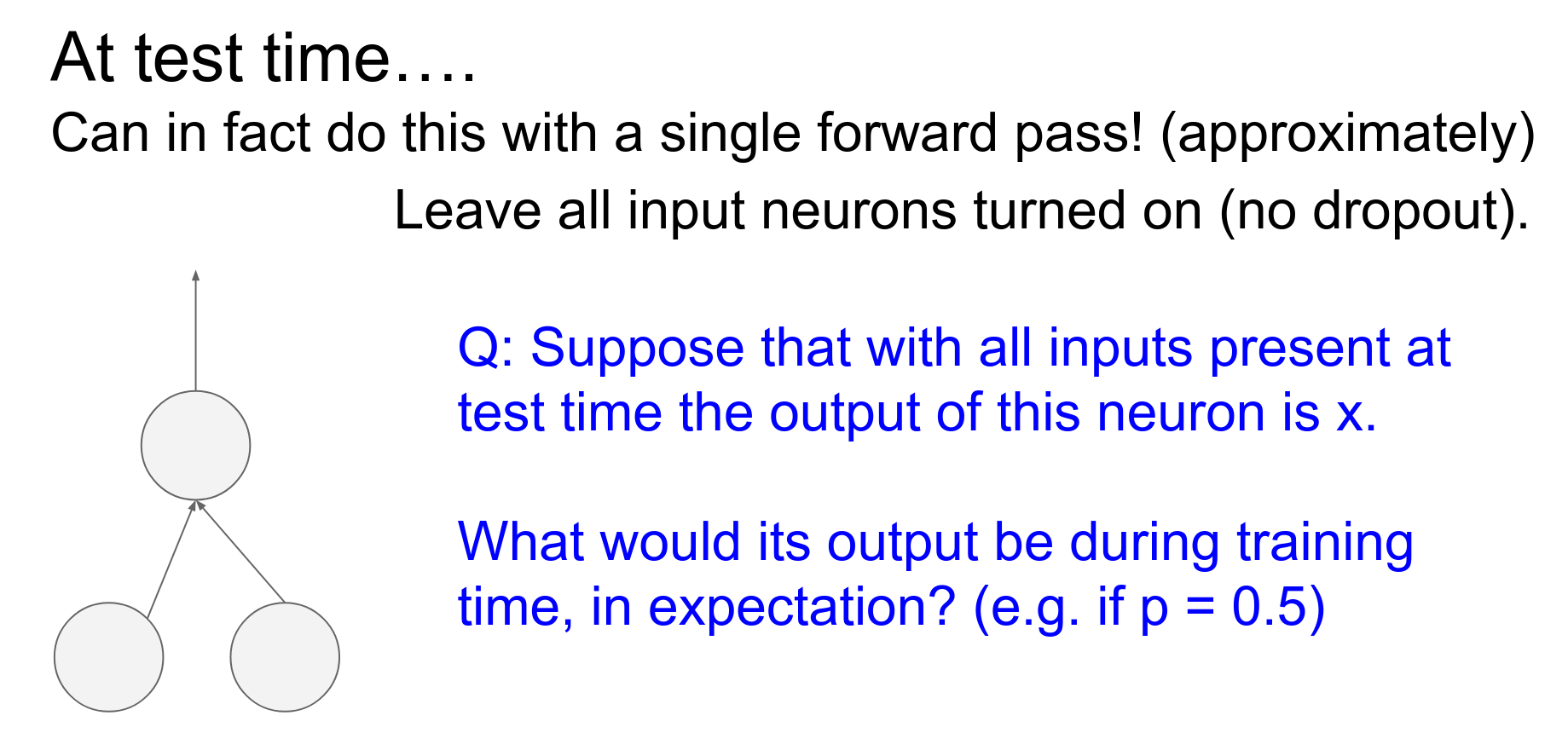
Can we use expectation?
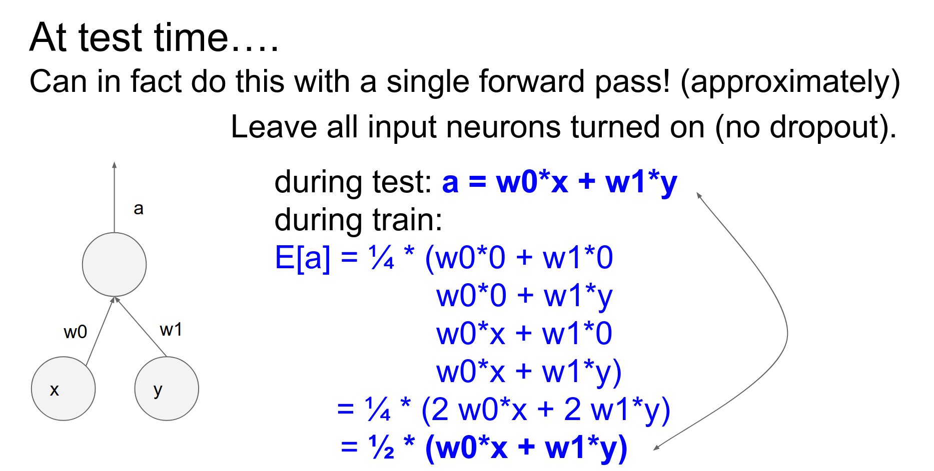
During testing, a linear neuron will give, in expectation, half of what it gives at training time.
That half comes from the half of the units we dropped.
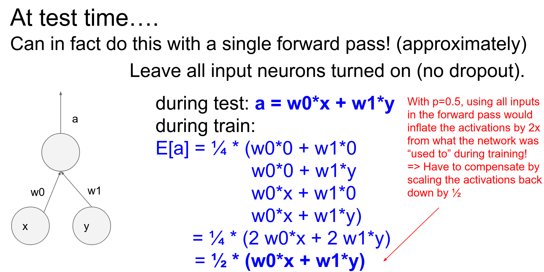
If we do not do this, we will end up having too large of an output compared to what we had in expectation at training time. Things will break in the NN, as they are not used to seeing such large outputs from the neurons.
Test Time Scaling
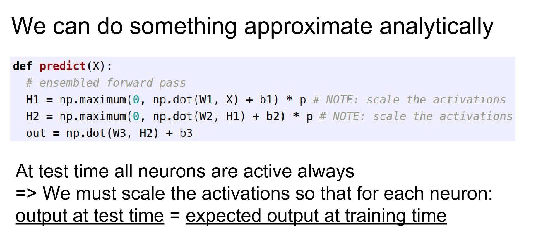
In this example, \(p\) can be \(0.5\).
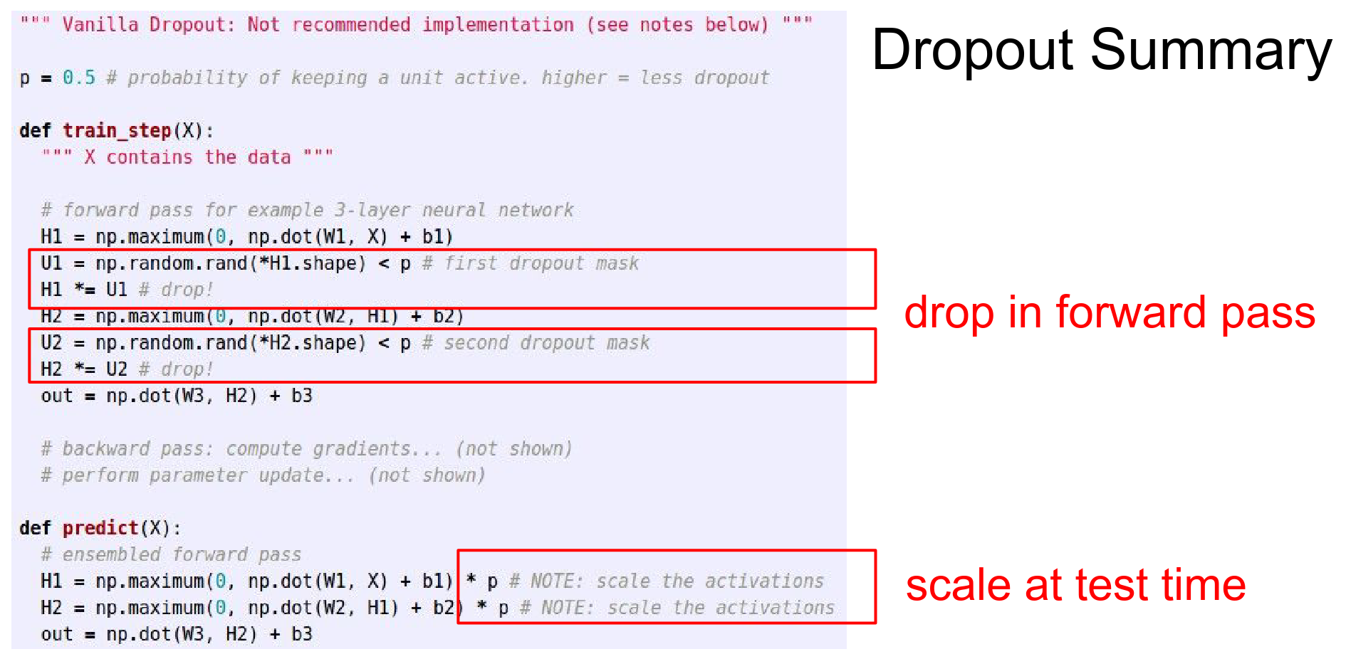
Do not forget to also backpropagate the masks.
Inverted Dropout
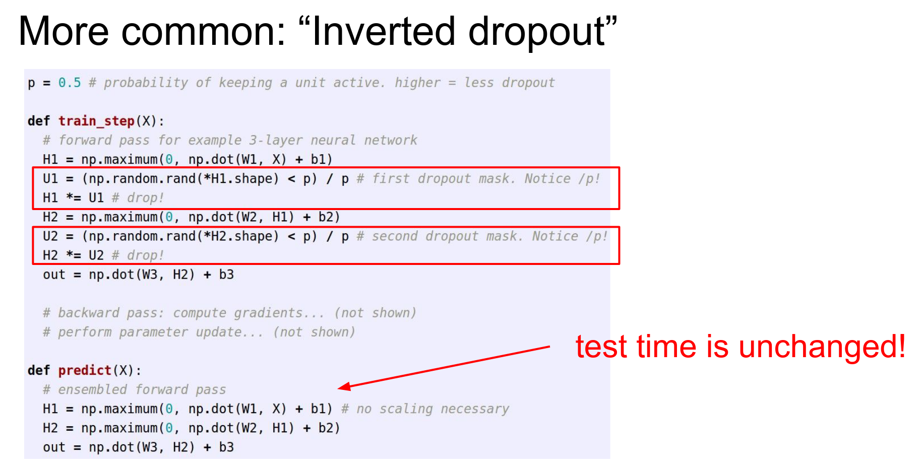
We select \(p\) each time we have a mini-batch.
Even though there is randomness in the exact amount of dropout, we still use 0.5.
Implement what you learn. Fast. Deep Learning Summer School Geoffrey Hinton.
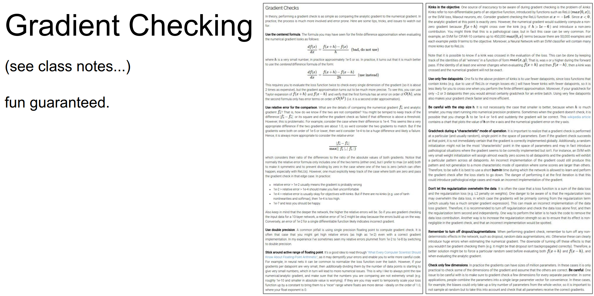
Go through the notes. Here is the link for it.
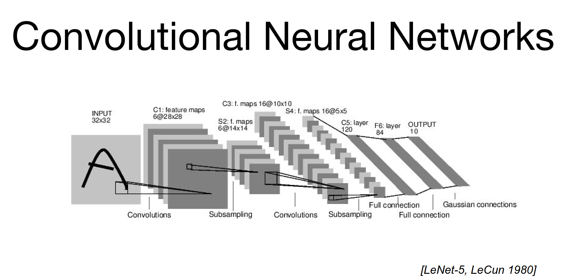
Convolutional Neural Networks
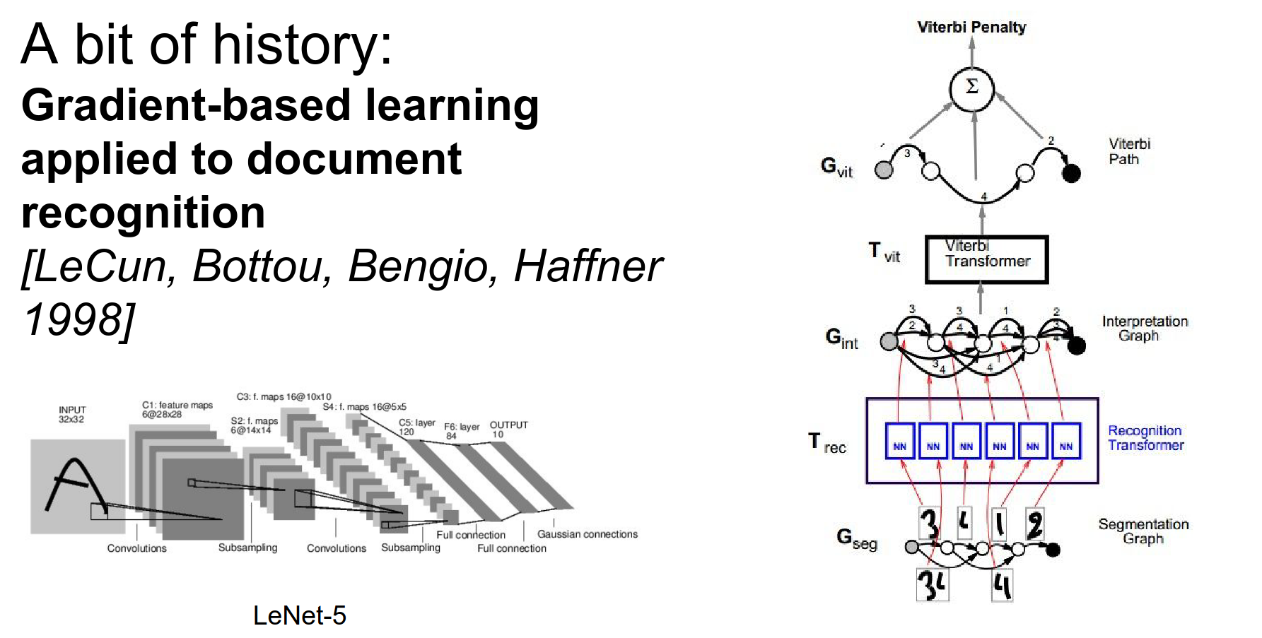
LeNet-5 - 1980.
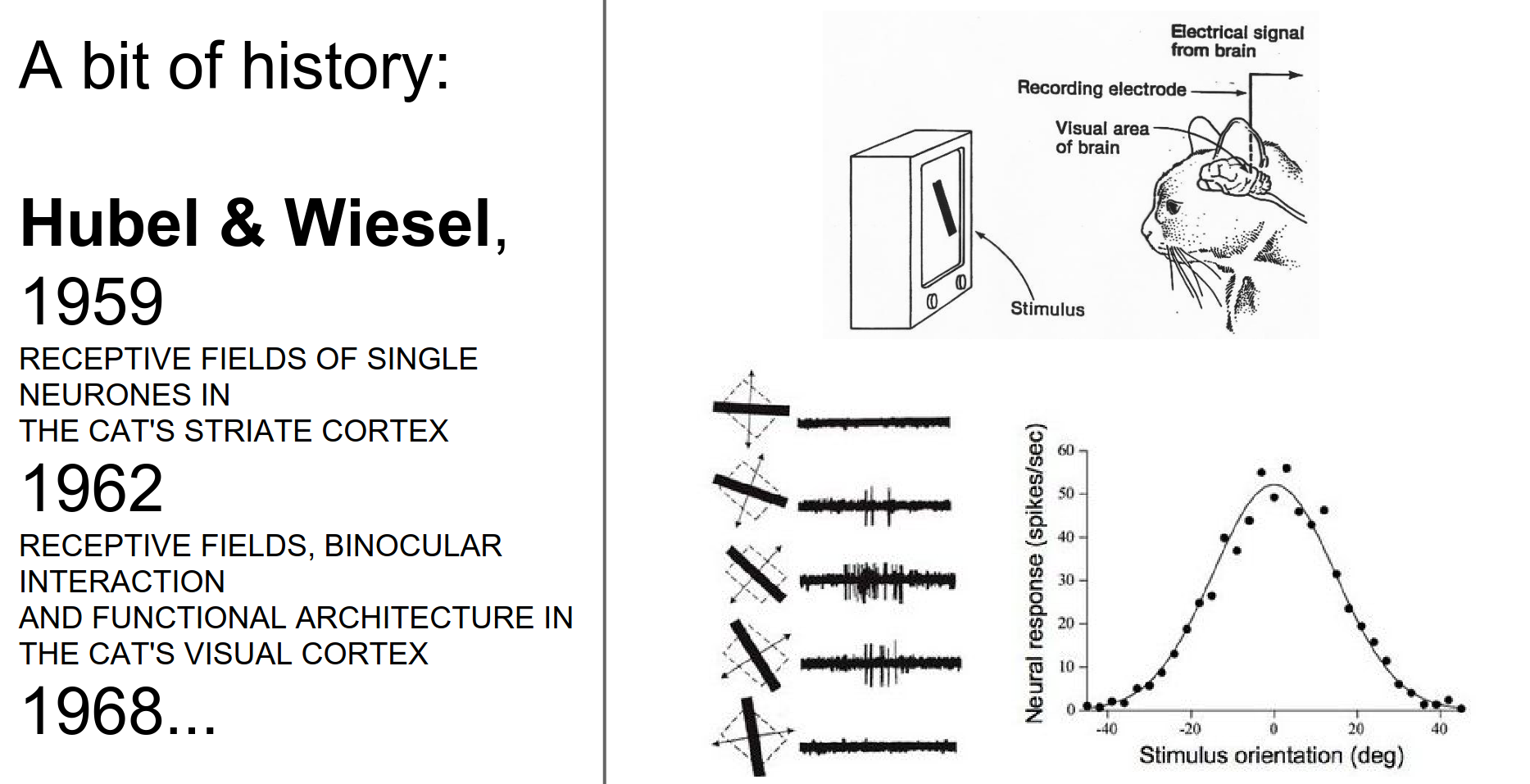
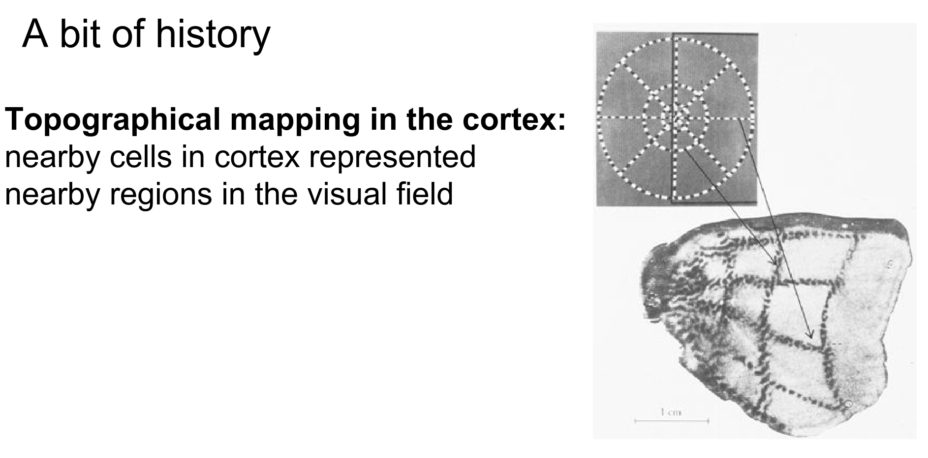
Fei Fei Li told us about this. Here is a video on the experiment.
This is one neuron in the V1 cortex. In a particular orientation, neurons get excited about edges.
Nearby cells in the visual cortex process nearby areas in your visual field. Locality is preserved in processing.
The visual cortex has a hierarchical organization, going from simple cells to complex cells through layers.
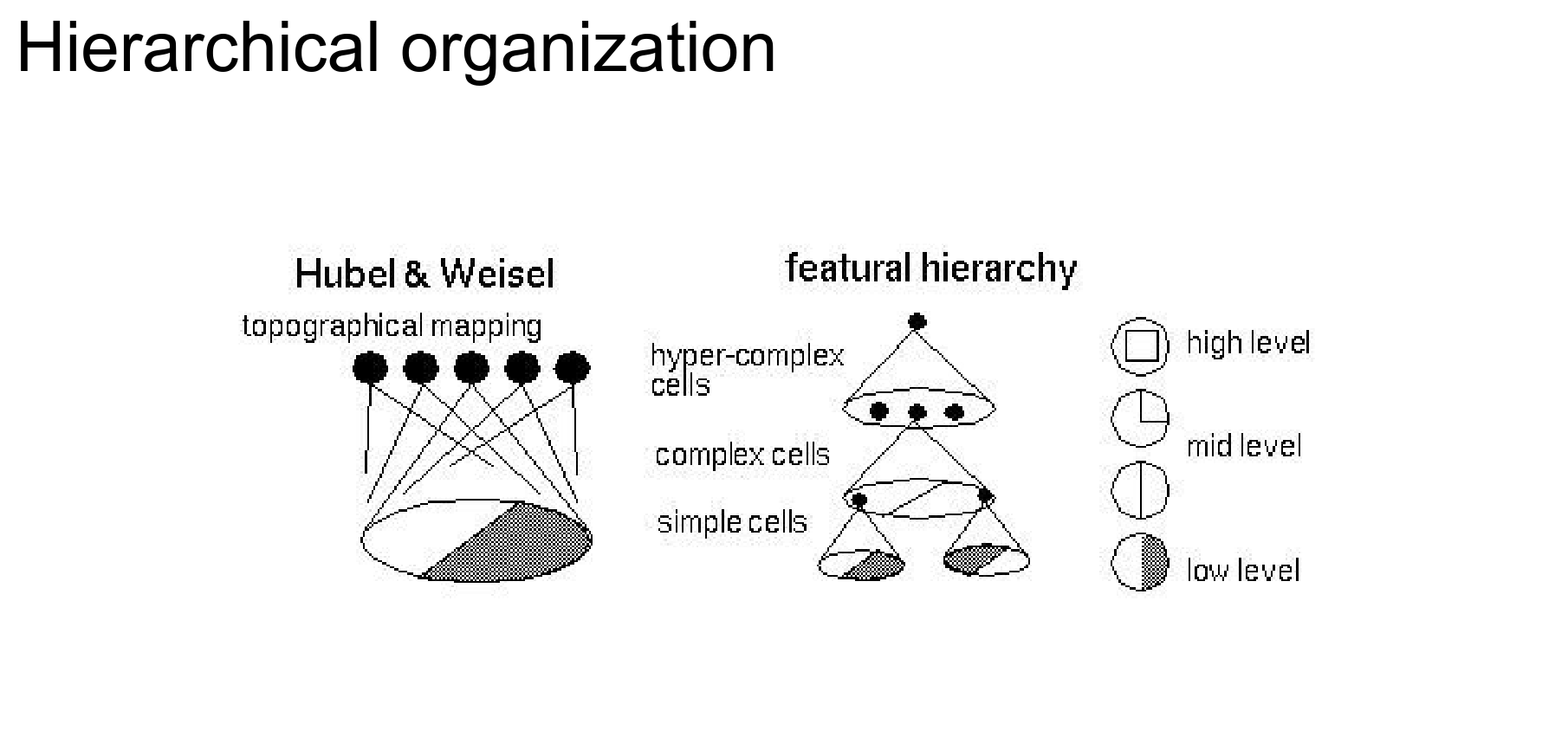
A layered architecture with these local receptive cells looks at a part of the input.
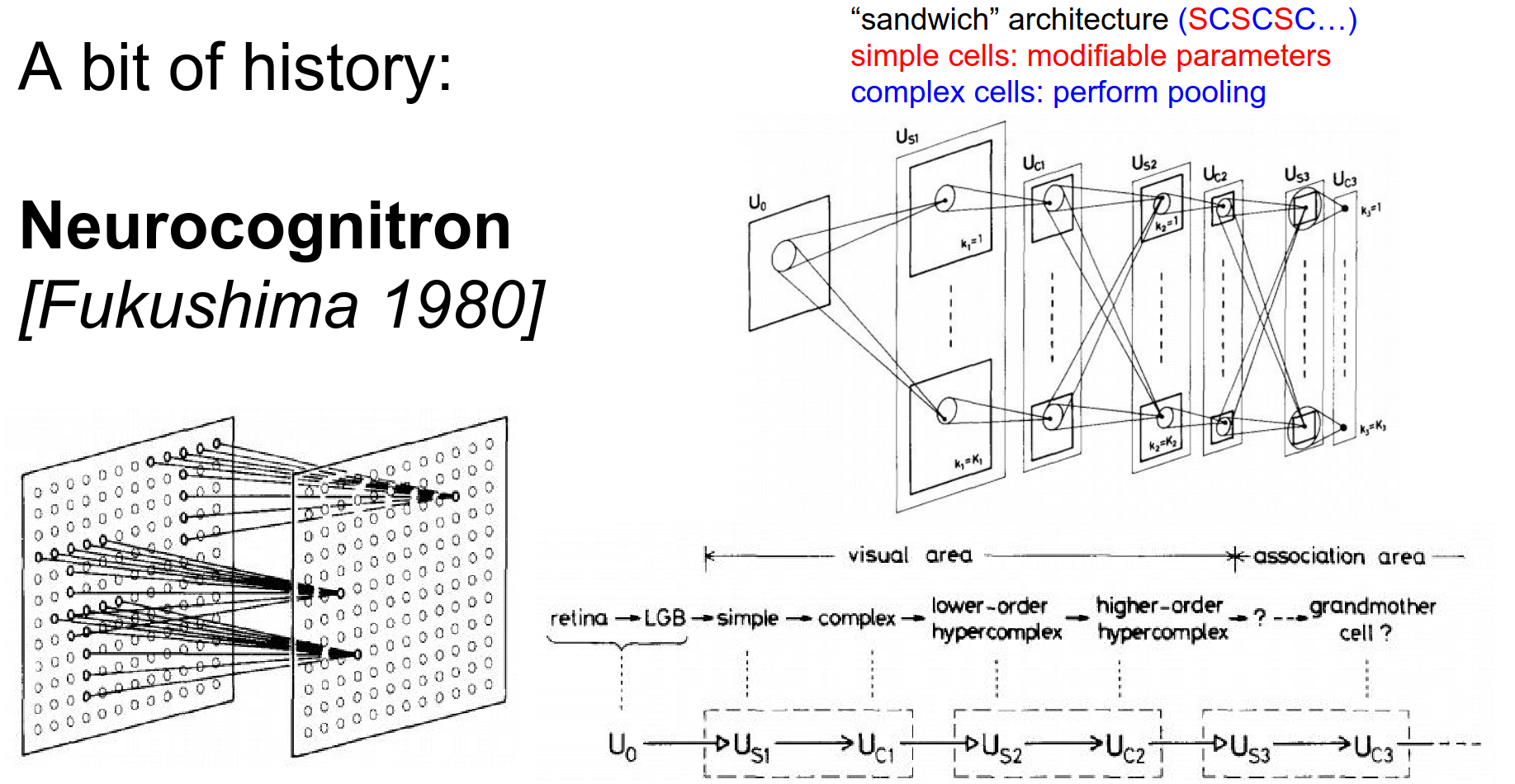
There was no backpropagation.
Yann LeCun built on top of this knowledge. He kept the rough architecture layout and trained the network using backpropagation.
AlexNet. In 2012, it won the ImageNet Challenge.
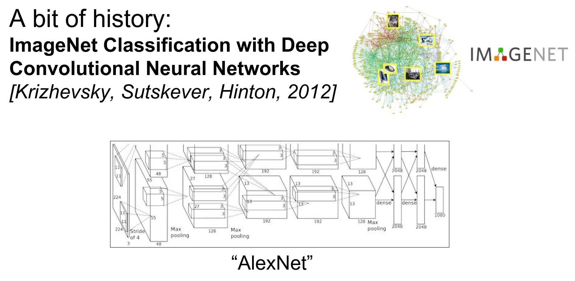
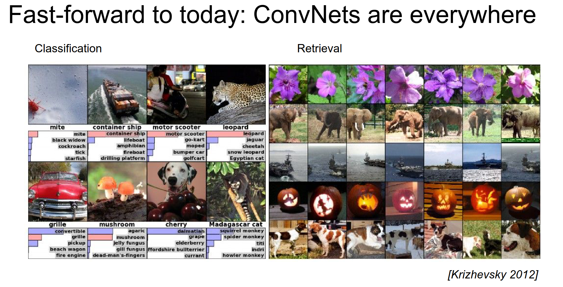
ConvNets can classify images.
They are really good at retrieval, showing similar images.
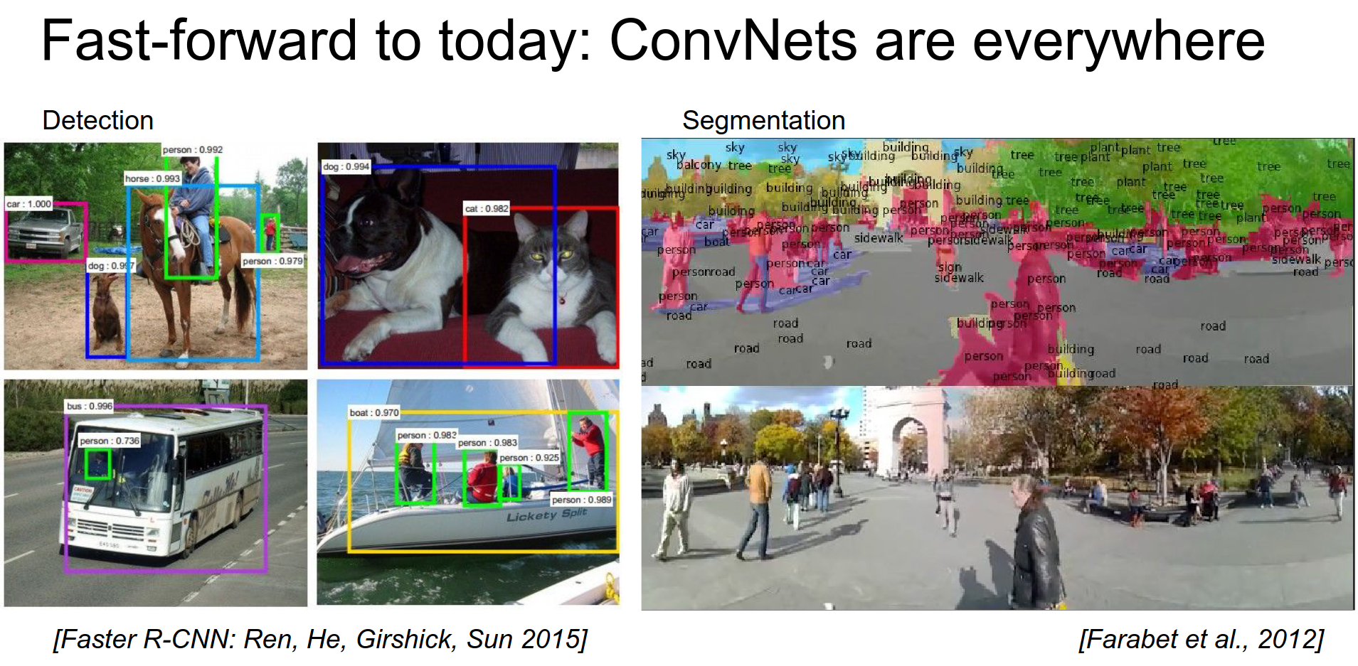
They can do detection.
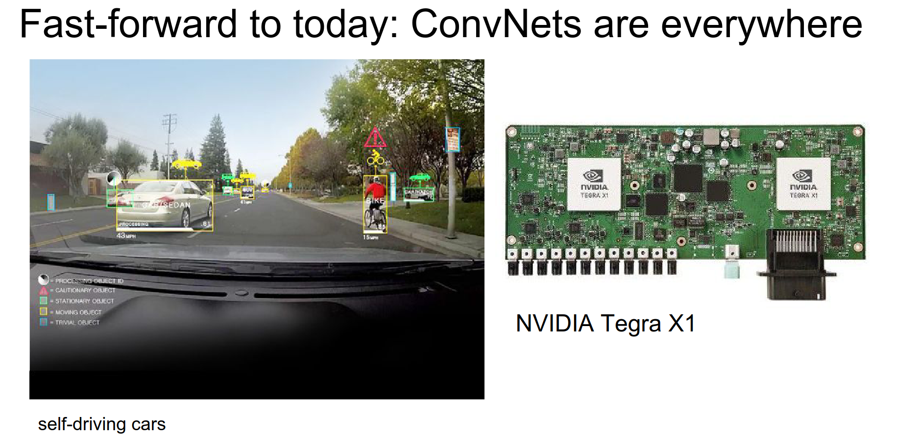
They are used in cars. You can do perception of things around you.
ConvNets are really good face detectors, like for tagging friends in Facebook.
Google is really interested in detecting street numbers.
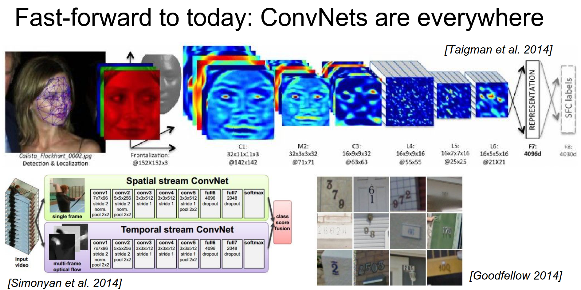
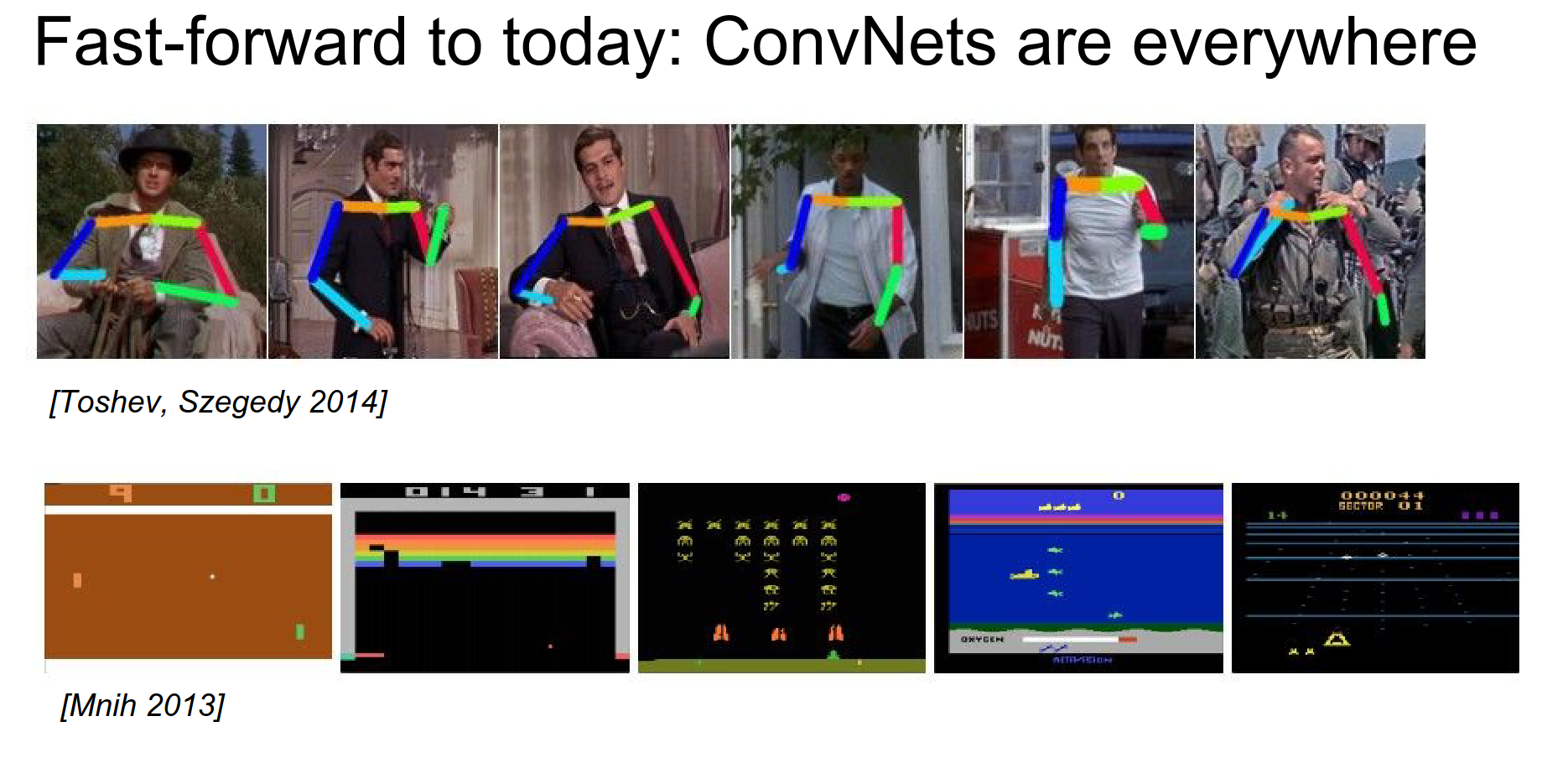
They can detect poses and play computer games.
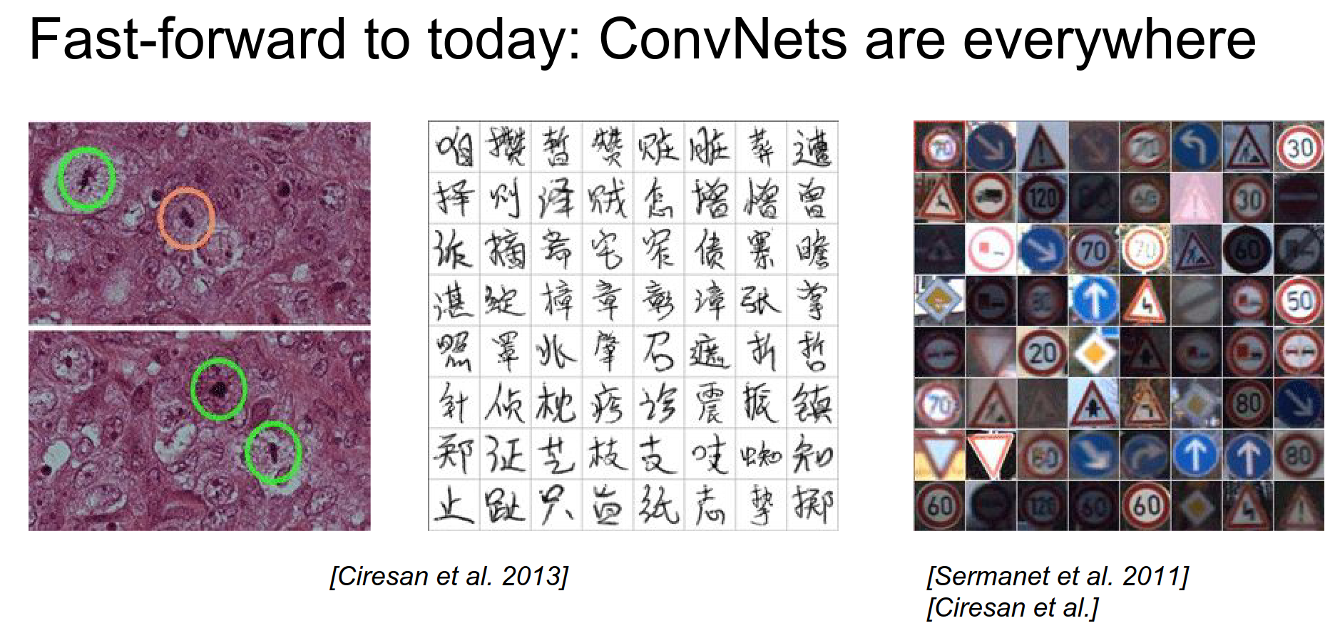
They can work on cells. They can read Chinese. They can recognize street signs.
They can recognize speech (a non-visual application). They can be used with text too.
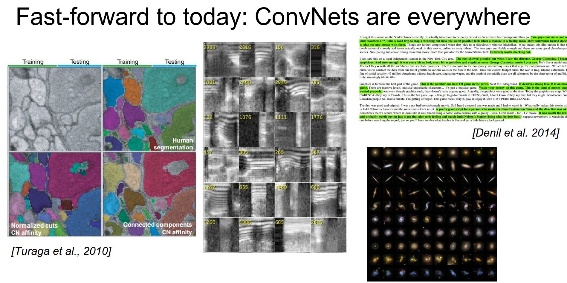
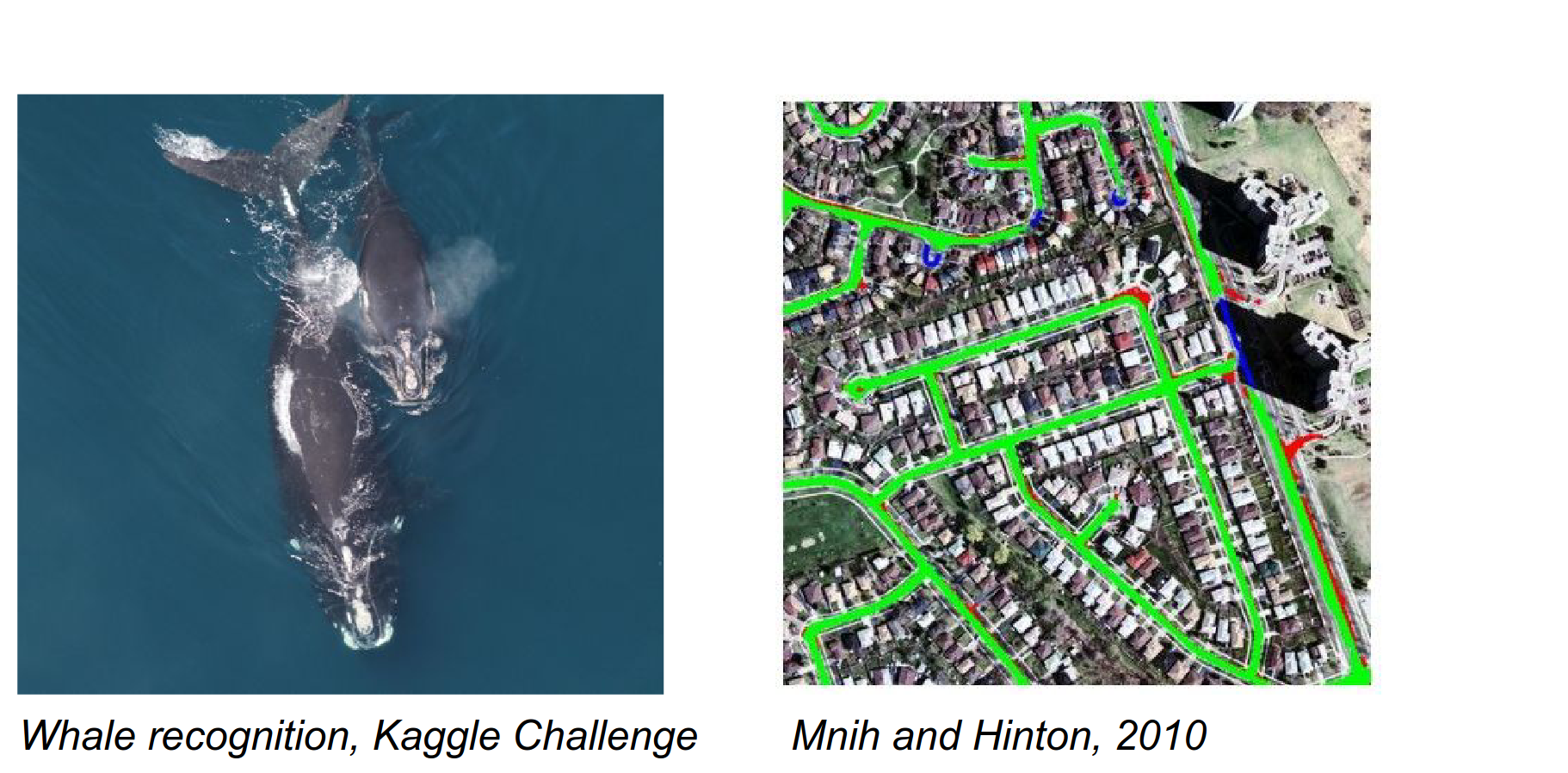
Specific types of whales. Satellite image analysis.
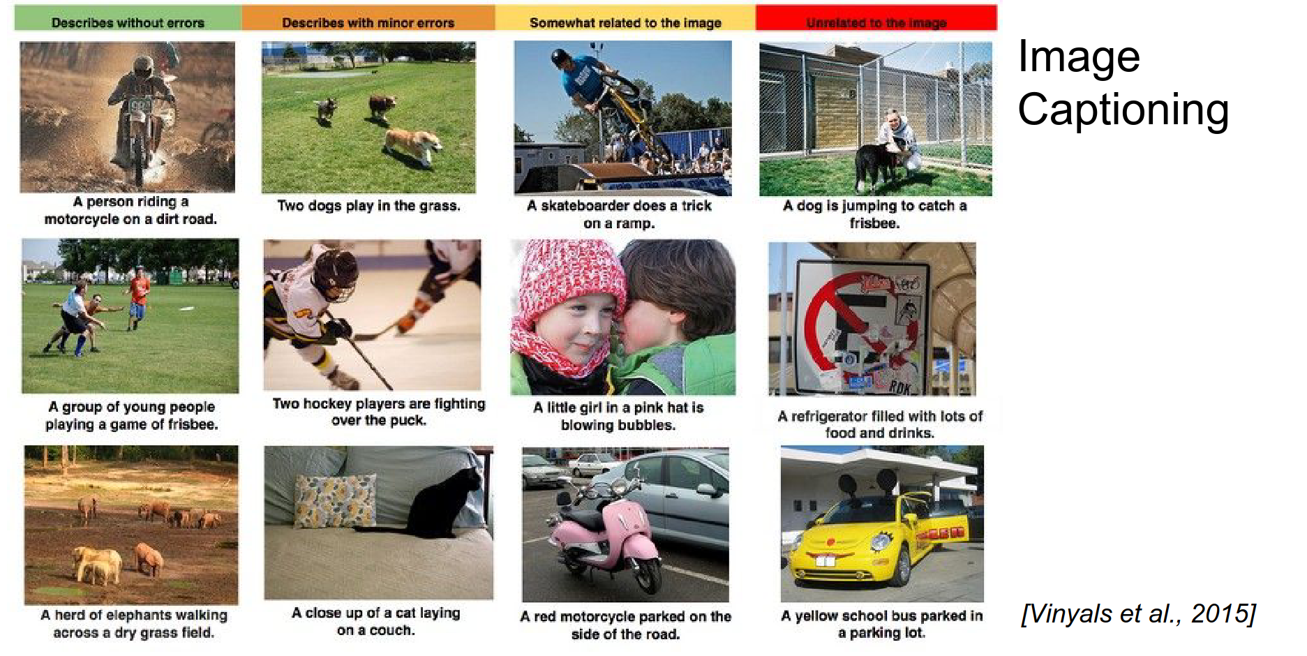
They can do image captioning.
They can do DeepDream. ImageNet has a lot of dogs, so they hallucinate dogs.
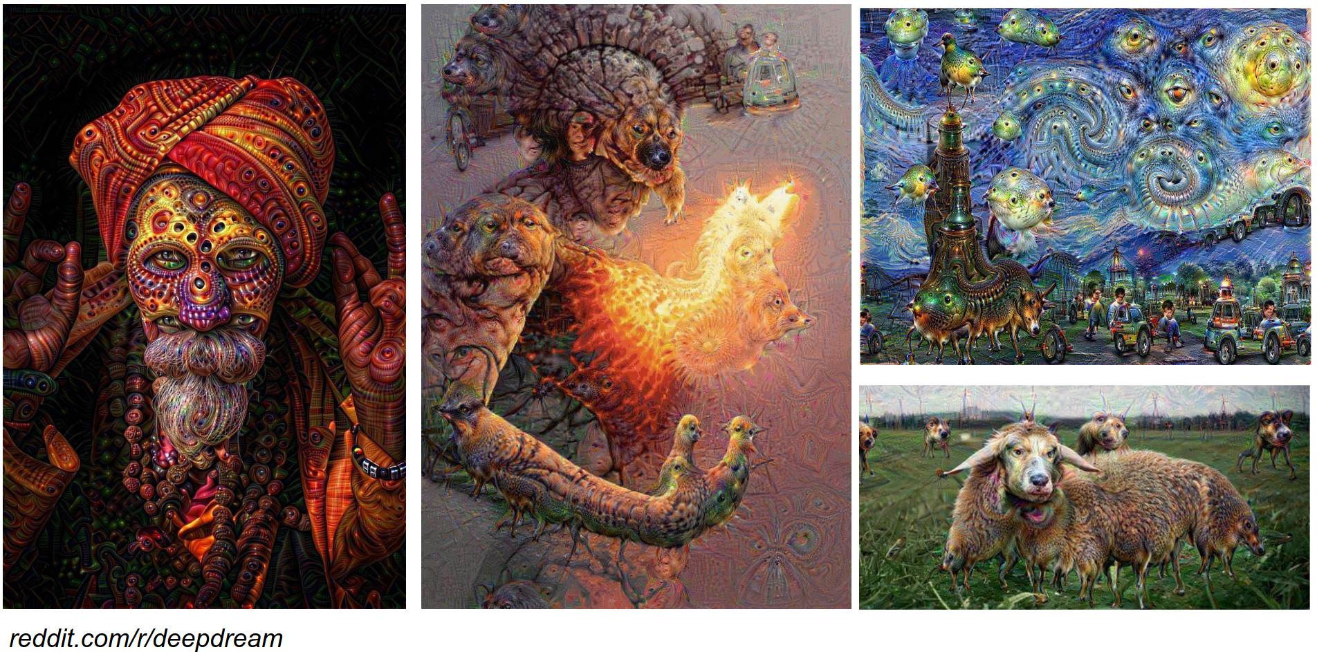
I will not explain this one.
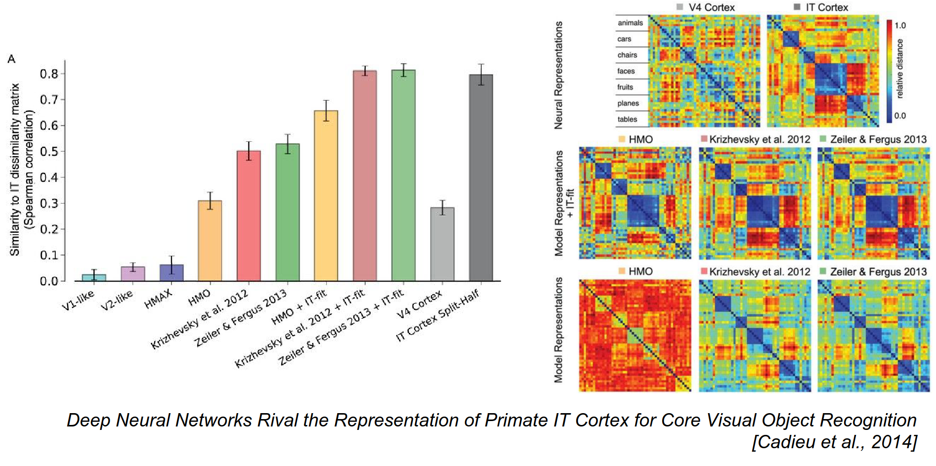
From an image, you can get results with a ConvNet almost equal to a monkey's IT Cortex.
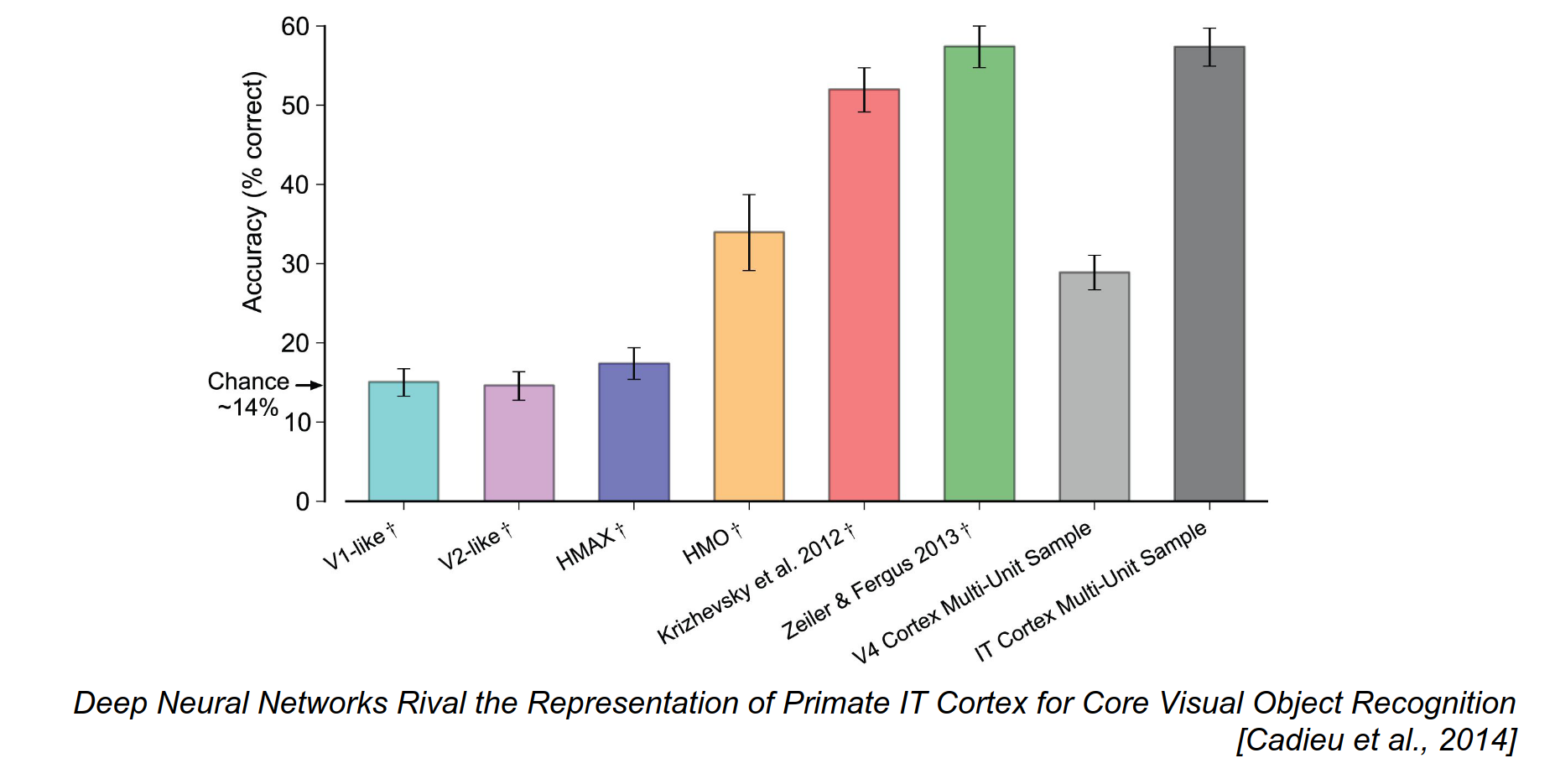
We show a lot of images to both the monkey and the ConvNet.
If you look at how images are represented in the brain and the ConvNet, the mapping is really, really similar.
How do they work?

Next class.