7. Convolutional Neural Networks

Part of CS231n Winter 2016

---

Lecture 7: Convolutional Neural Networks

Two weeks to go on Assignment 2.

Project Proposal? About Project

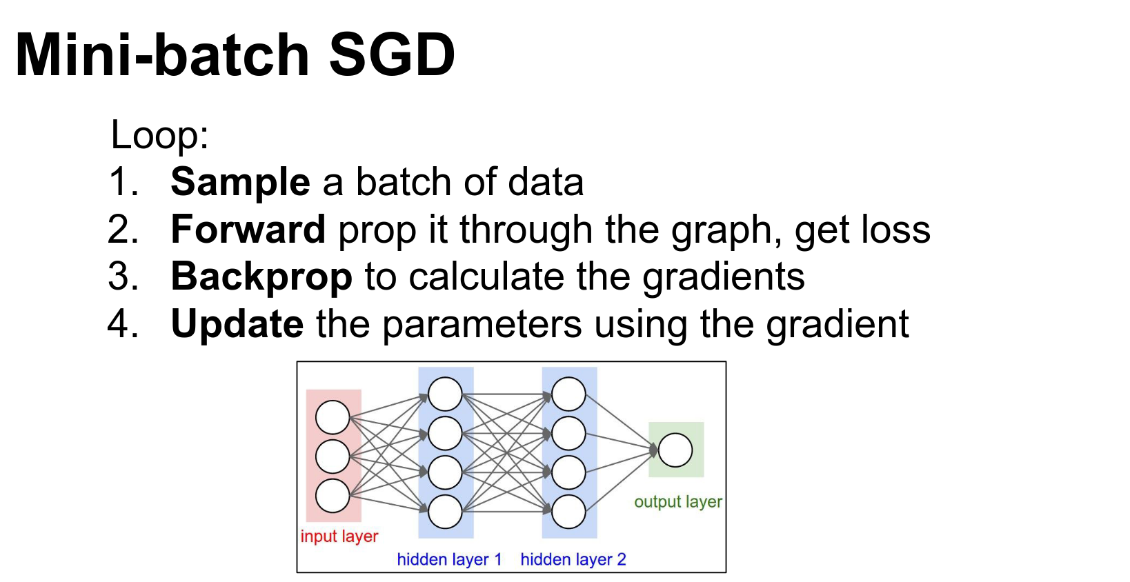
The four-step process is still relevant.

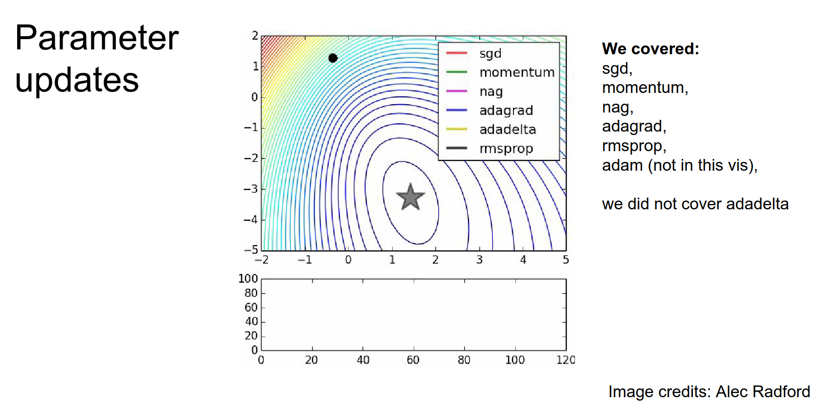
How did we update parameters?

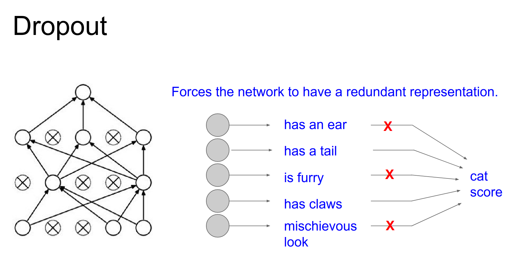
Dropout was casually introduced by Geoffrey Hinton.

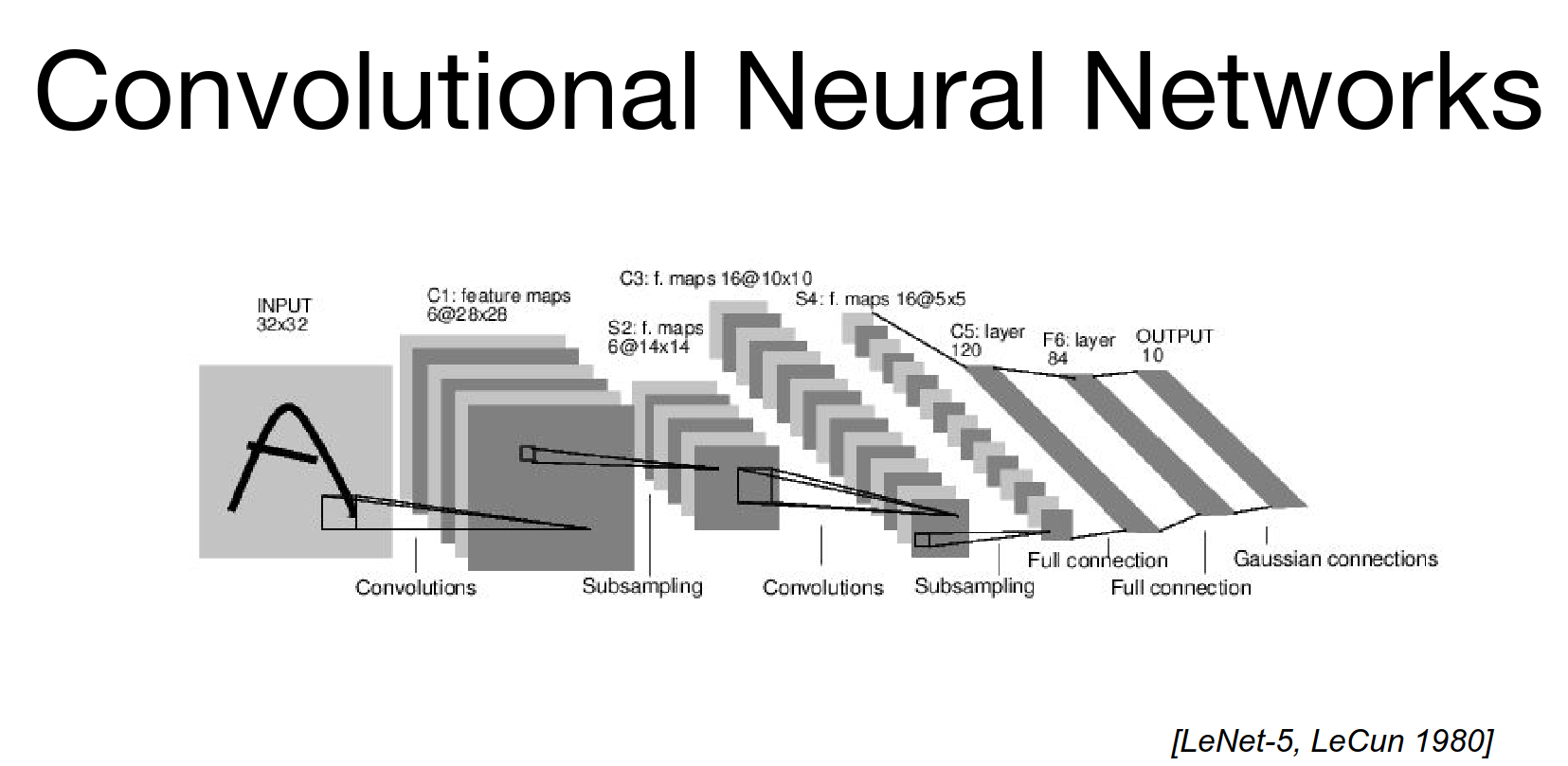
LeNet is a classic architecture.

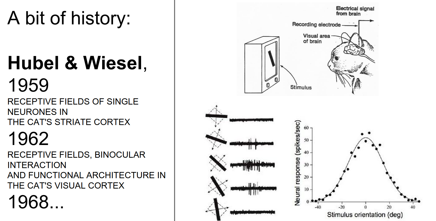
Hubel and Wiesel's experiments.

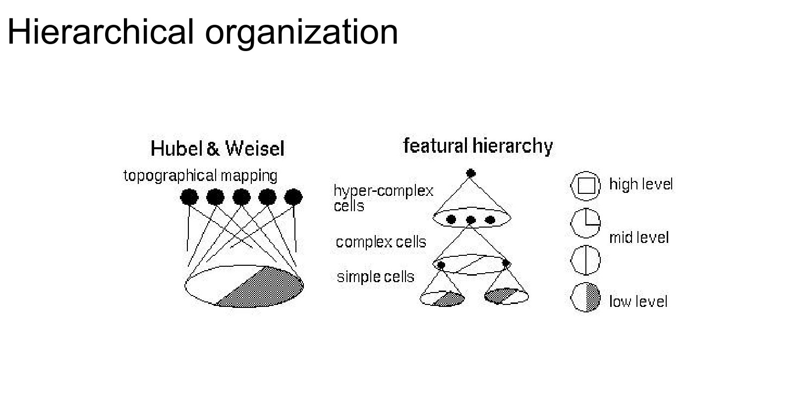
Feature hierarchy.

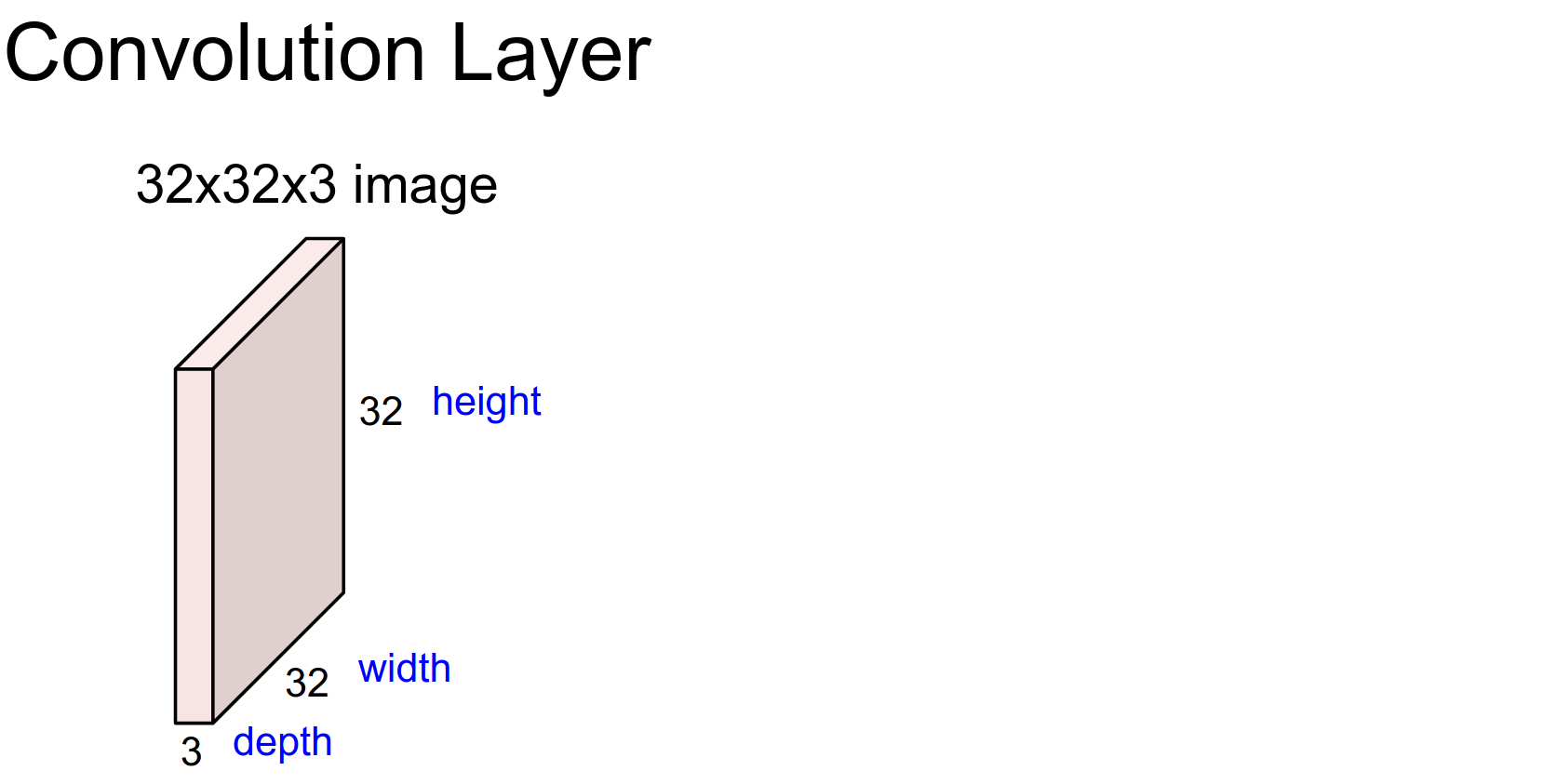
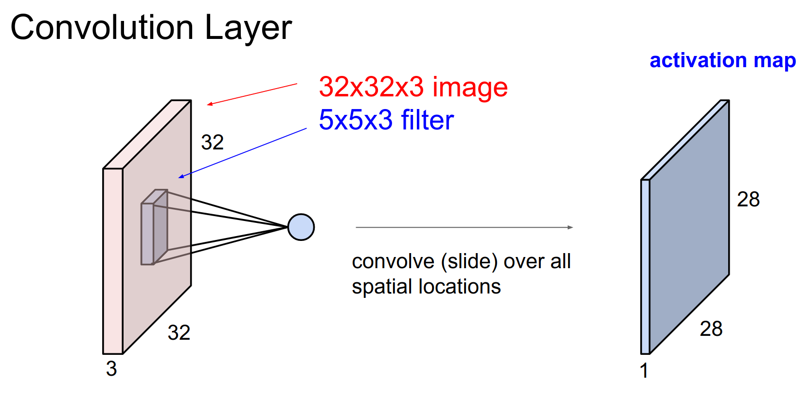
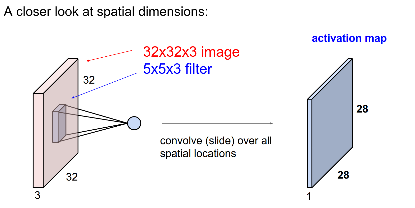
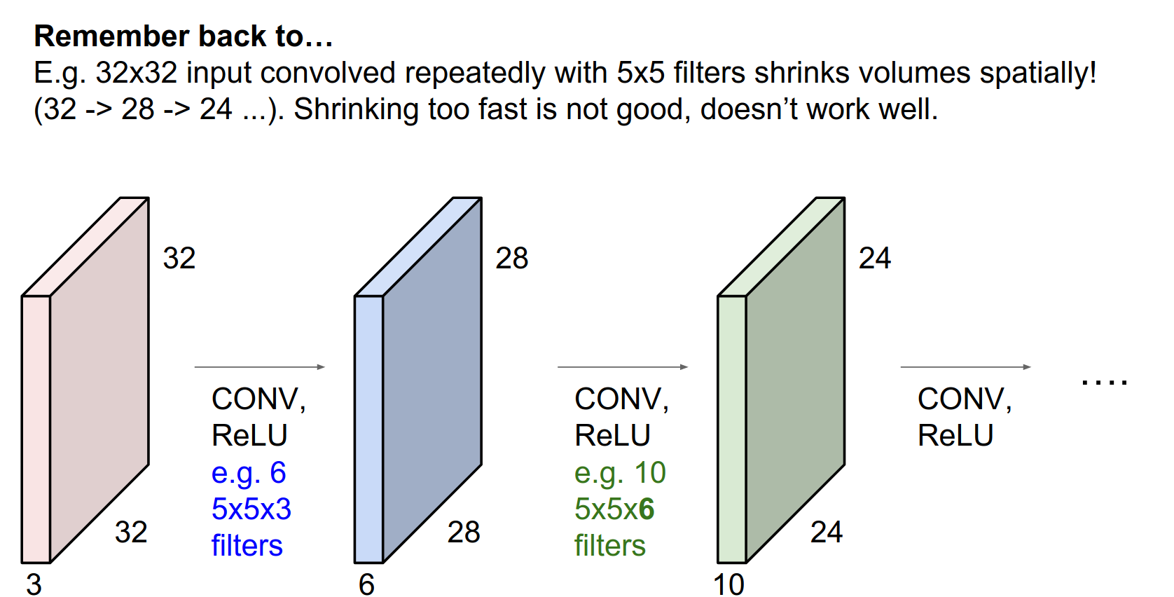
We start with a \(32x32x3\) CIFAR-10 image.

It has 3 channels, so the volume of activations is 3 deep. This corresponds to the 3rd dimension of the volume.

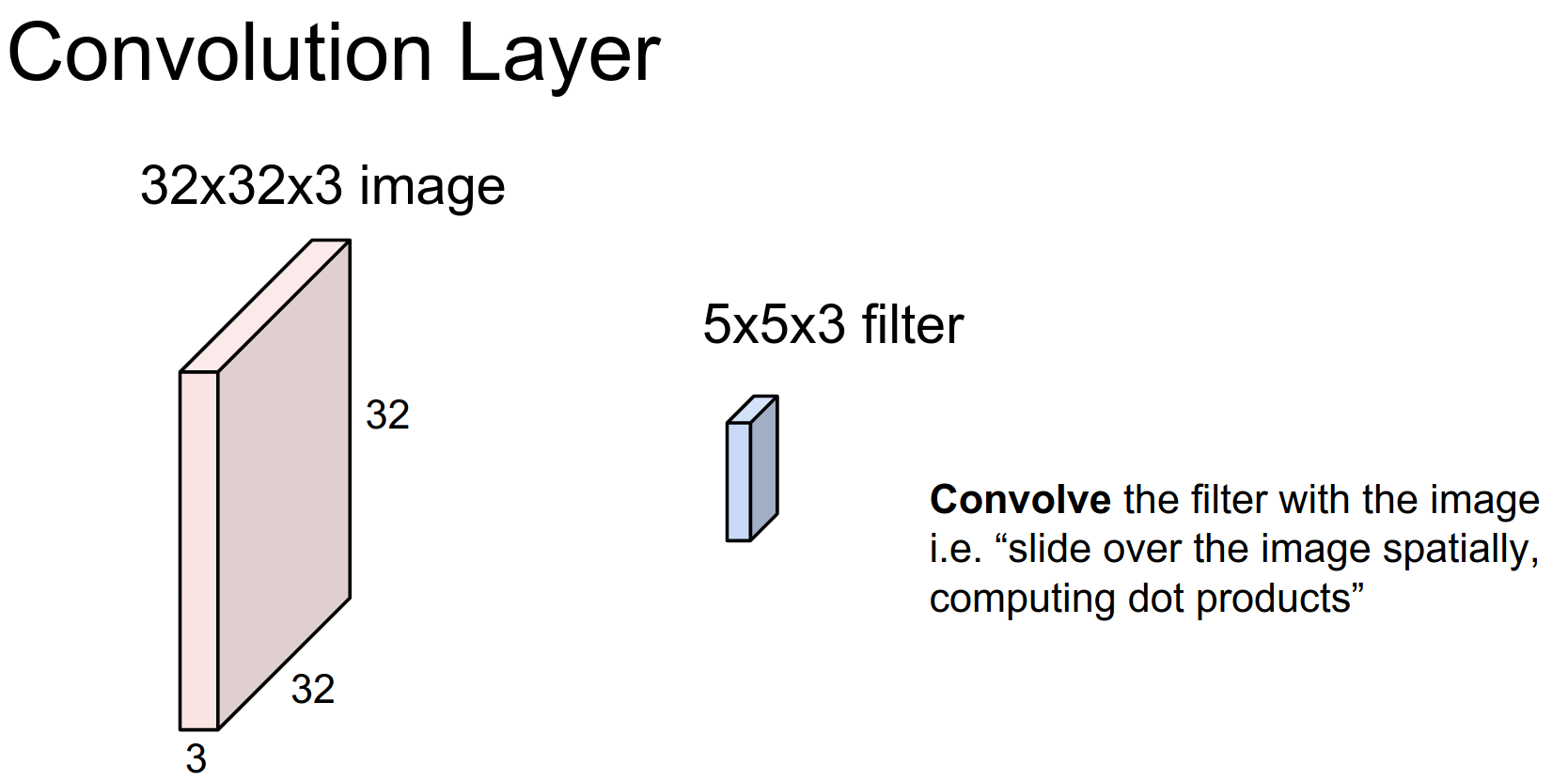
Convolutional Layer: A core building block.

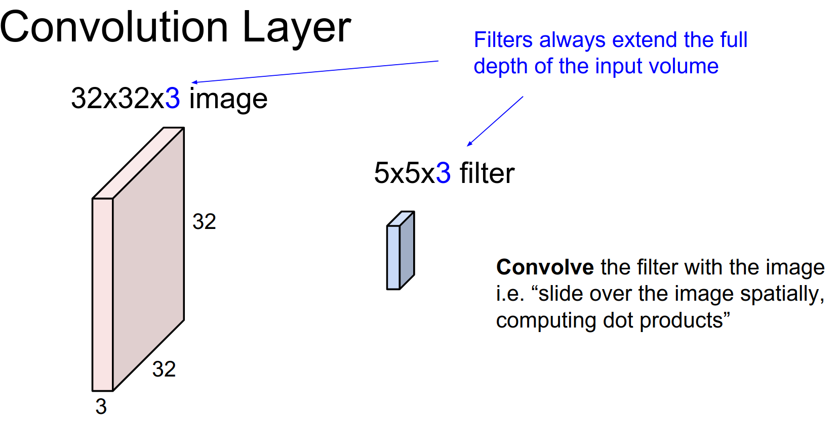
A filter with a depth of 3 will cover the full depth of the input volume. However, it is spatially small (\(5x5\)).

We always extend through the full depth of the input volume.

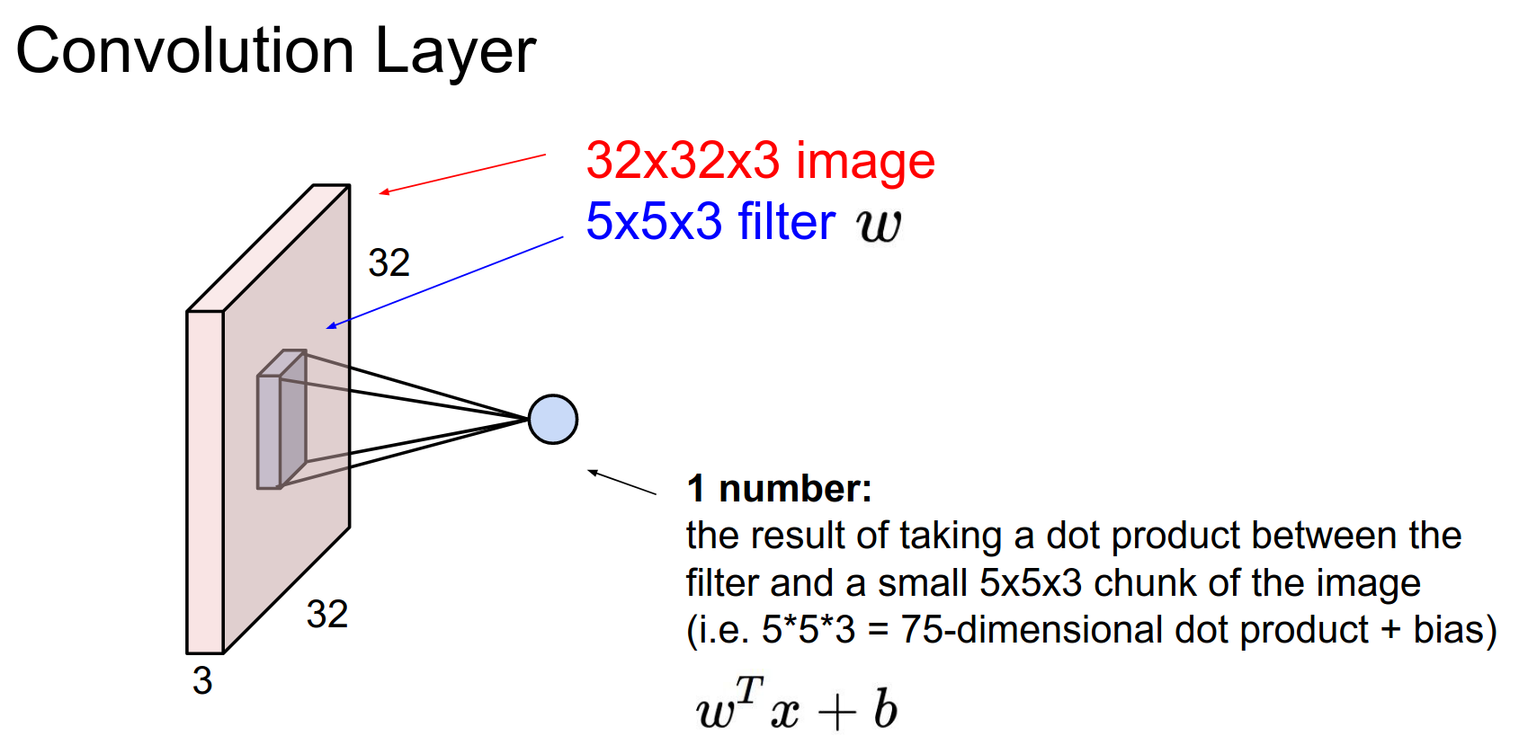
We will learn \(w\). We are going to slide the filter over the input volume.

As we slide, we perform a 75-dimensional dot product.

This sliding process results in an activation map.

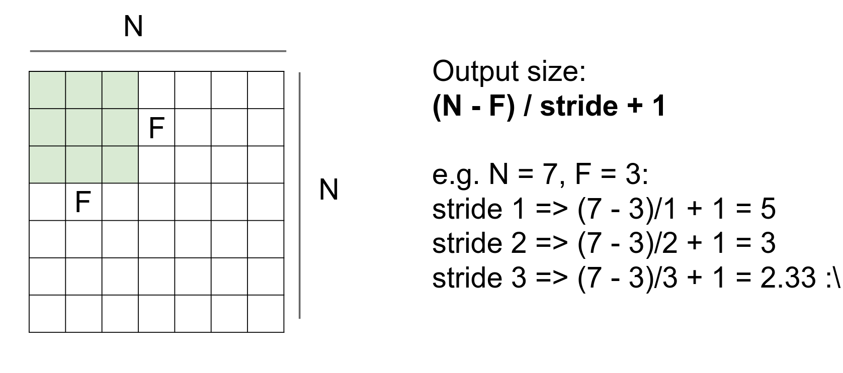
Activation Map Size

Because we slide the filter from index 0 to 4 on the input image, we can place the filter in 28x28 distinct locations.

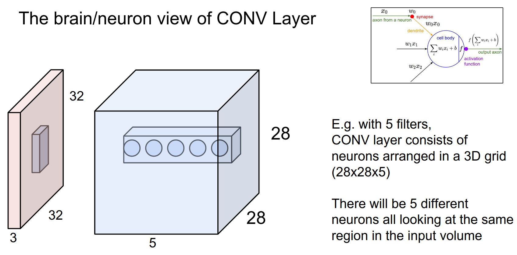
We will actually have a filter bank. Different filters will result in different activation maps.

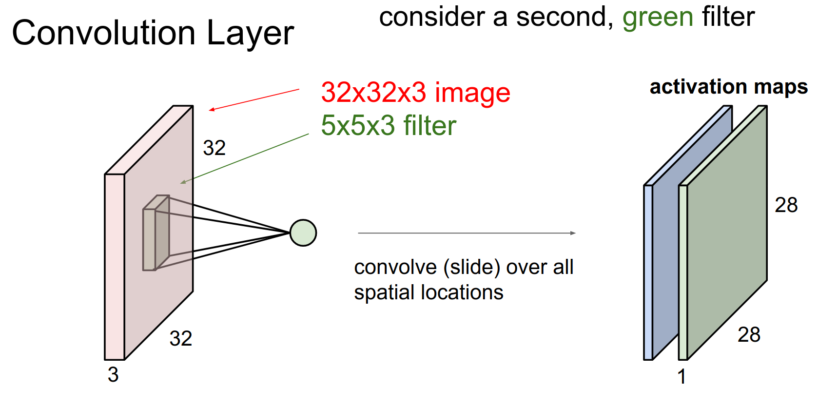
6 filters will result in 6 activation maps.

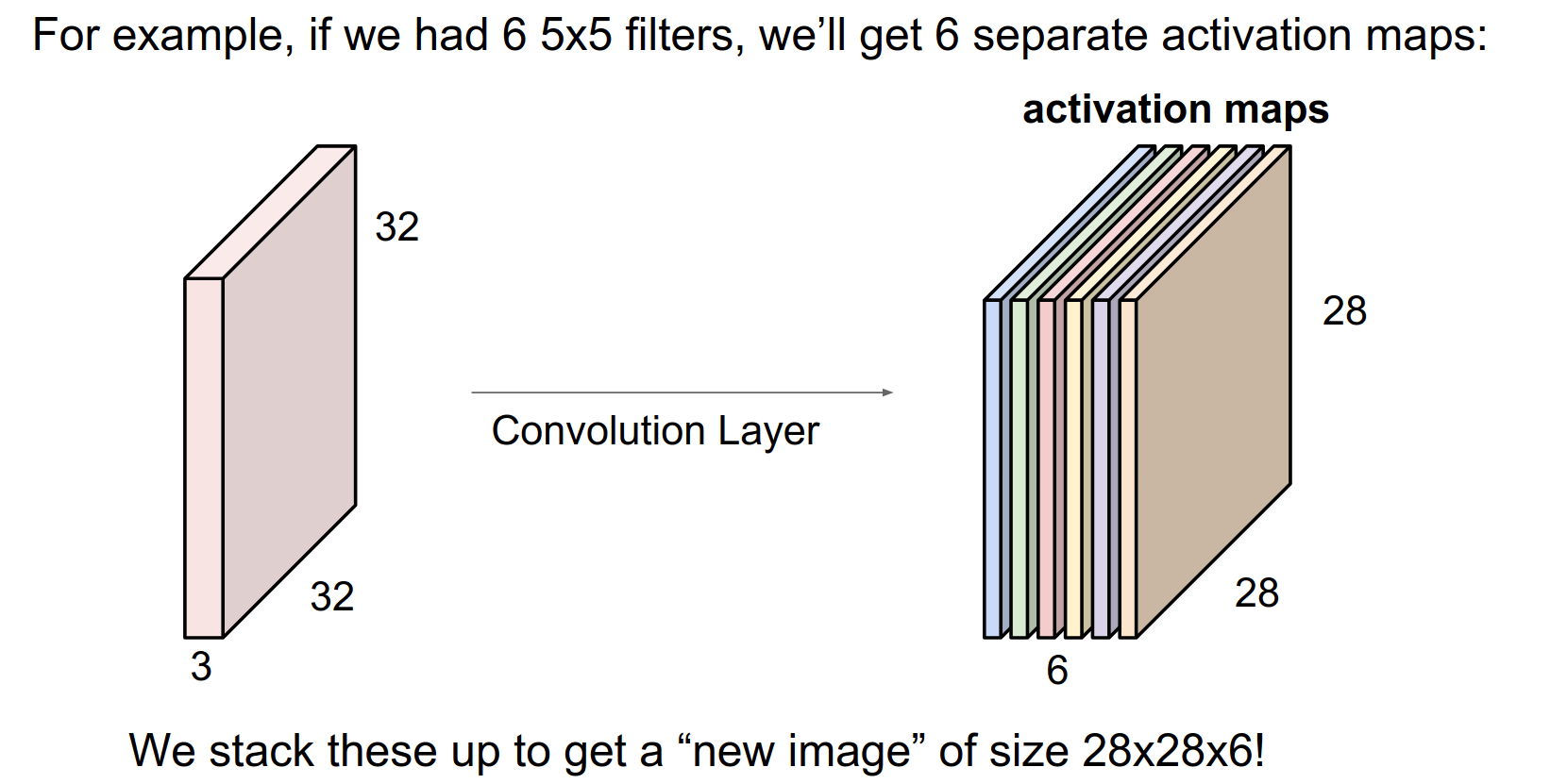
Output Dimensions

After all the convolutions, we will have a new image sized \(28x28x6\)!

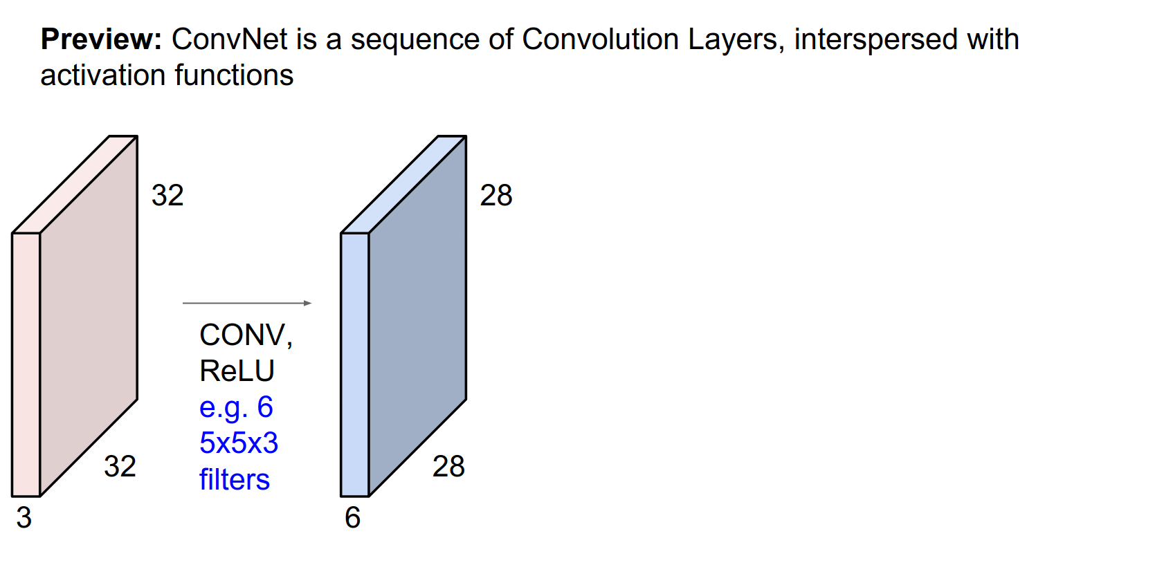
We will have these convolutional layers, which will have a certain number of filters. These filters will have a specific spatial extent (e.g., 5x5). This conv layer will slide over the input and produce a new image. This will be followed by a ReLU and another conv layer.

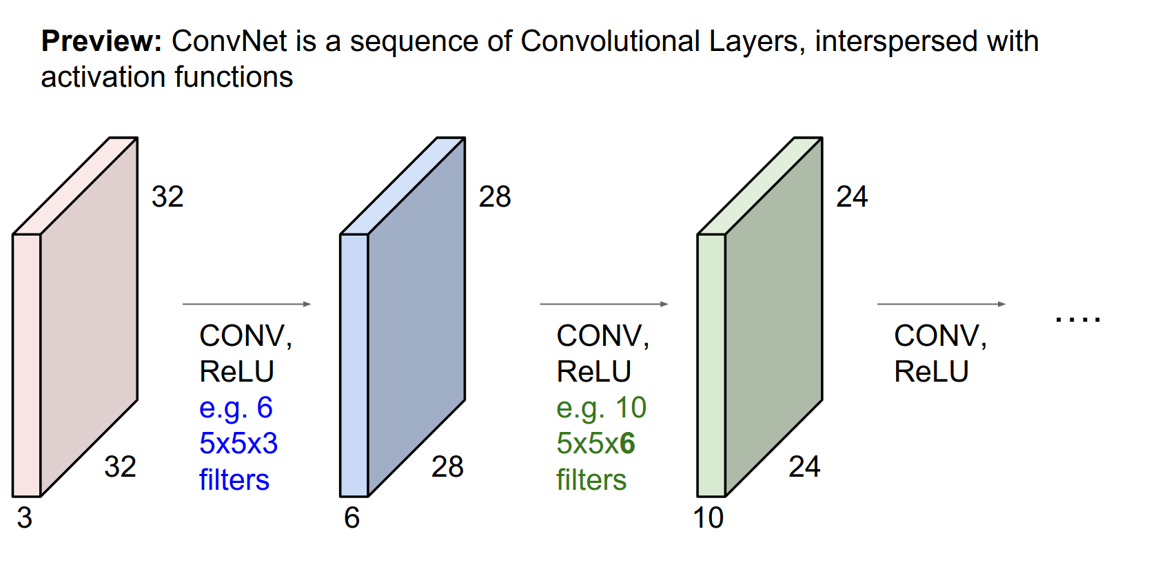
The filters now have to be \(5x5x6\).

Input Depth Matching

These filters are initialized randomly. They will become the parameters in our ConvNet.

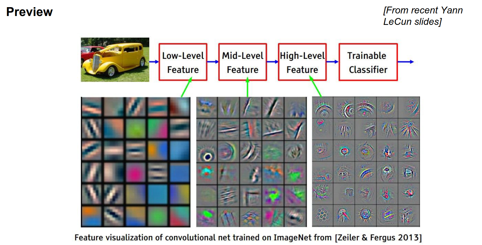
When you look at the trained layers, the first layers represent low-level features: color pieces, edges, and blobs.

The first layers will look for these features in the input image as we convolve through it.

As you go deeper, we perform convolution on top of convolution, doing dot products over the outputs of the previous conv layer.

It will put together all the color/edge pieces, making larger and larger features that the neurons will respond to.

For example, mid-level layers might look for circles.

And in the end, we will build object templates and high-level features.

In the leftmost picture, these are raw weights (\(5x5x3\) array).

In the middle and right, these are visualizations of what those layers are responding to in the original image.

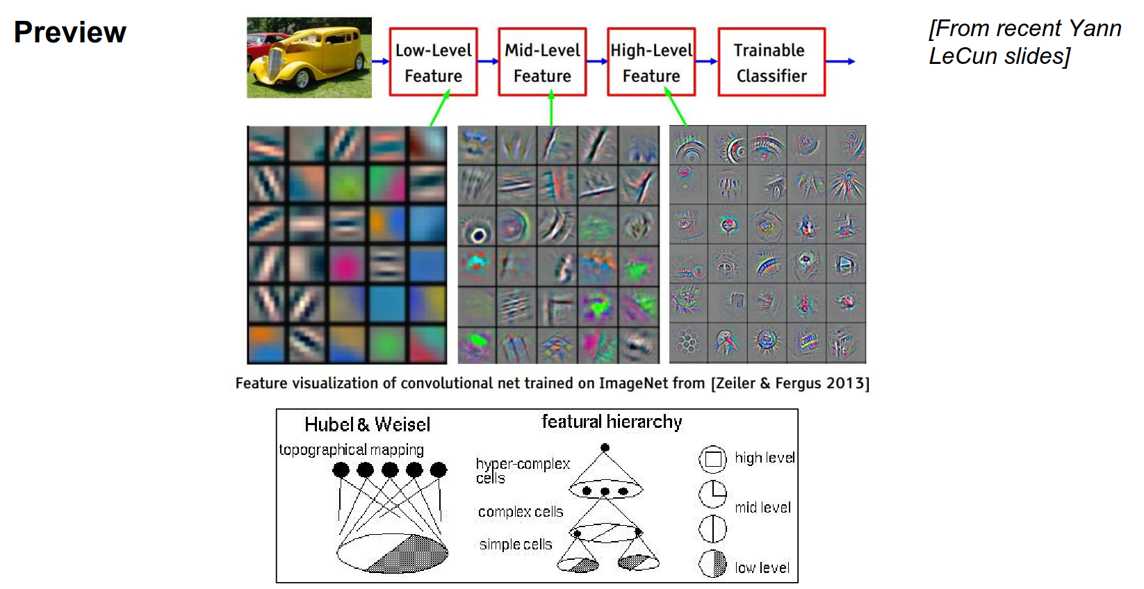
This is pretty similar to what Hubel and Wiesel imagined: a bar of a specific orientation leads to more complex features.

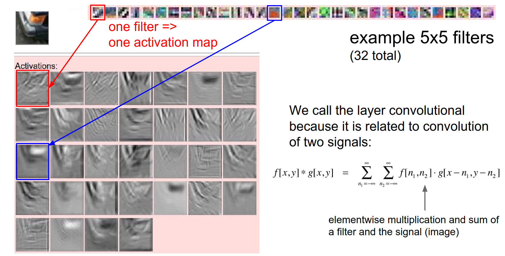
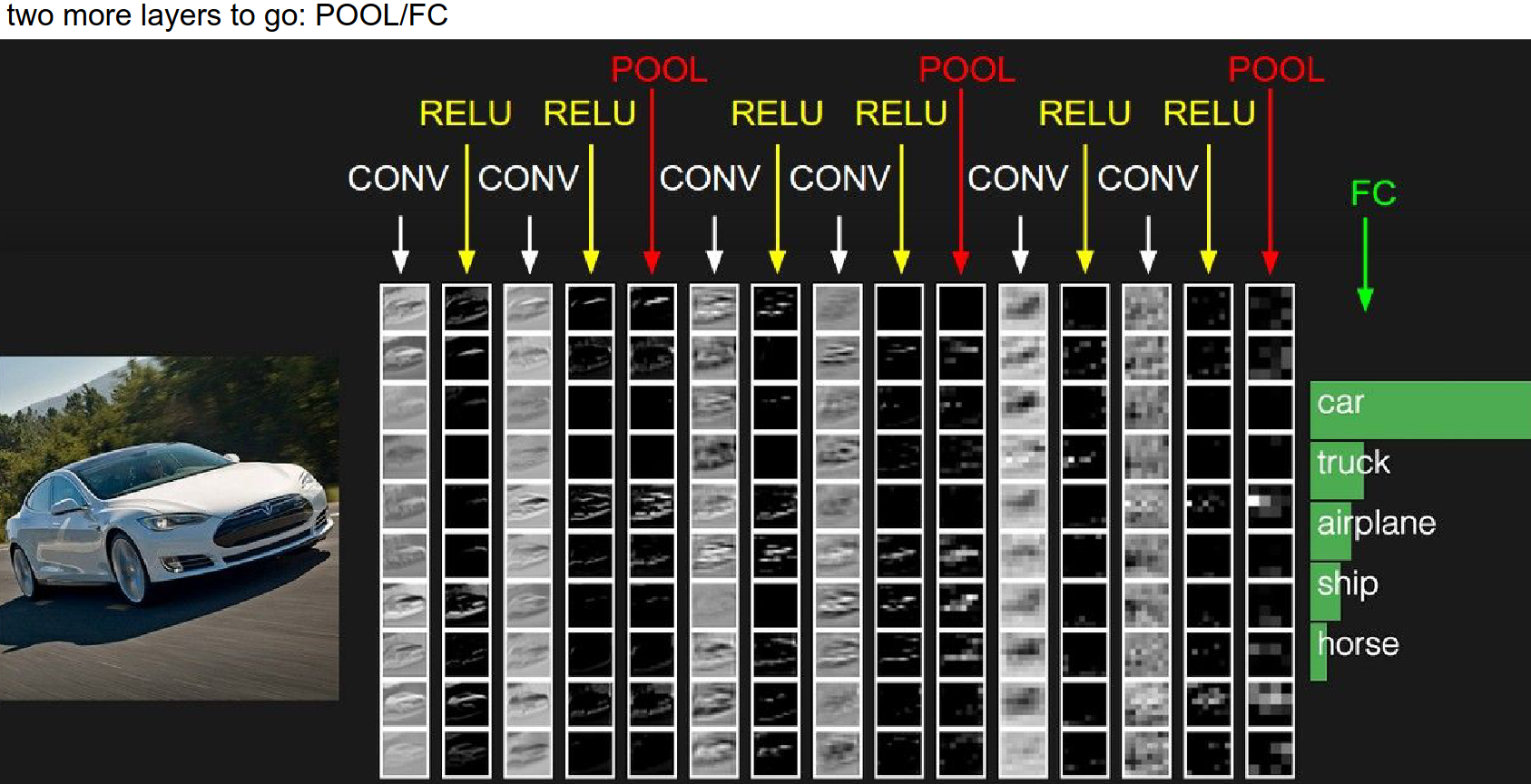
A small piece of a car as input.

32 filters of size 5x5 in the first convolutional layer.

Below are example activation maps. White corresponds to high activation, and black corresponds to low activation (low numbers).

Where the blue arrow points to orange stuff in the image, the activation shows that the filter is happy about that part.

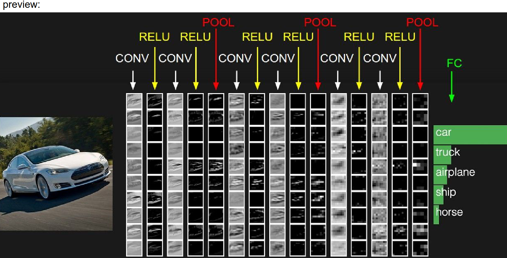
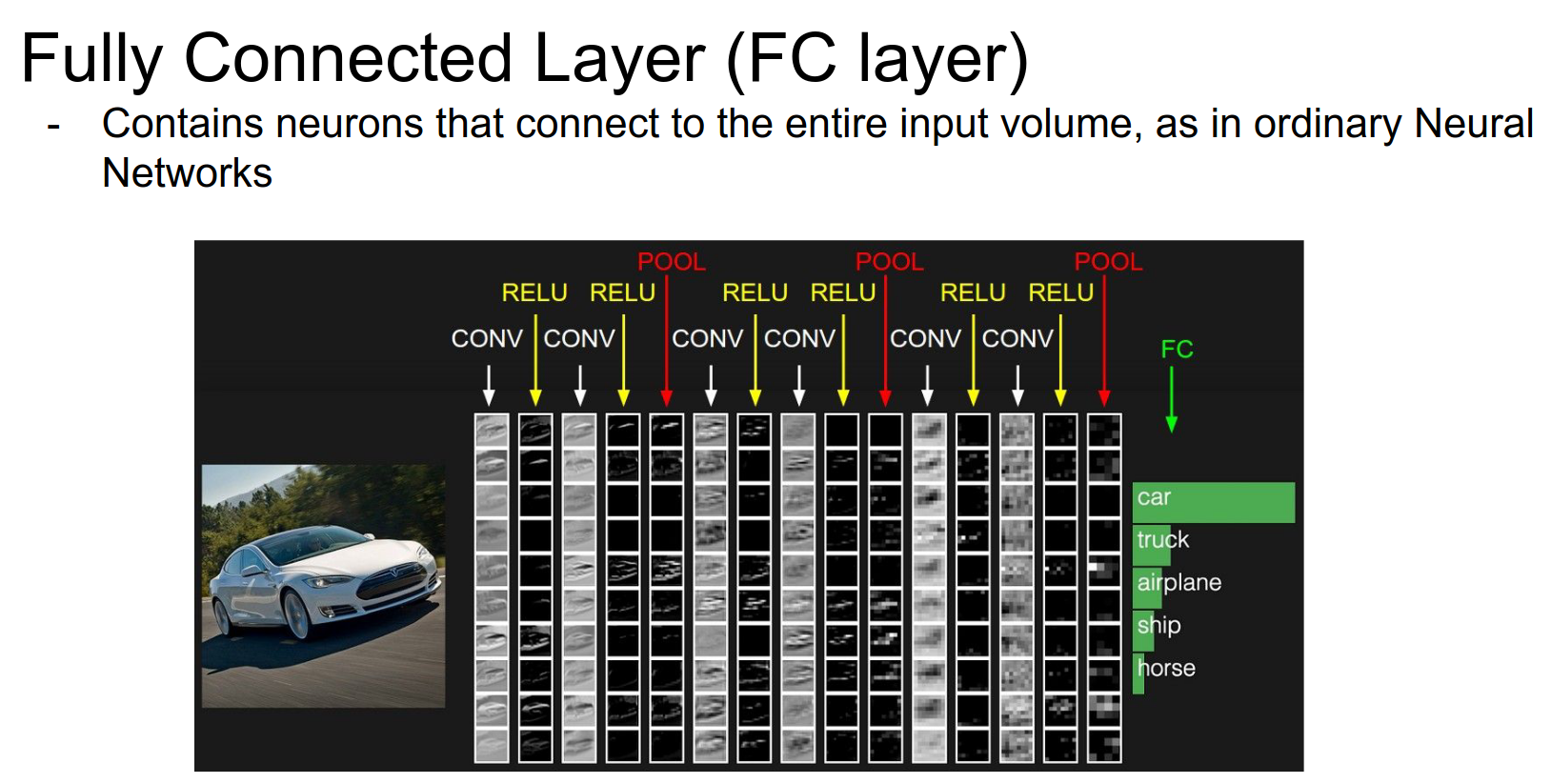
A layout like this:

Architecture Overview

Also, a Fully Connected layer at the end.

Every row is an activation map. Every column is an operation.

ReLU Layer

The image feeds into the left side. We do convolution, thresholding (ReLU), then another Conv, another ReLU, then pooling...

Piece by piece, we create these 3D volumes of higher and higher abstraction. We end up with a volume connected to a large FC layer.

The last matrix multiplication will give us the class scores.

Filter Count

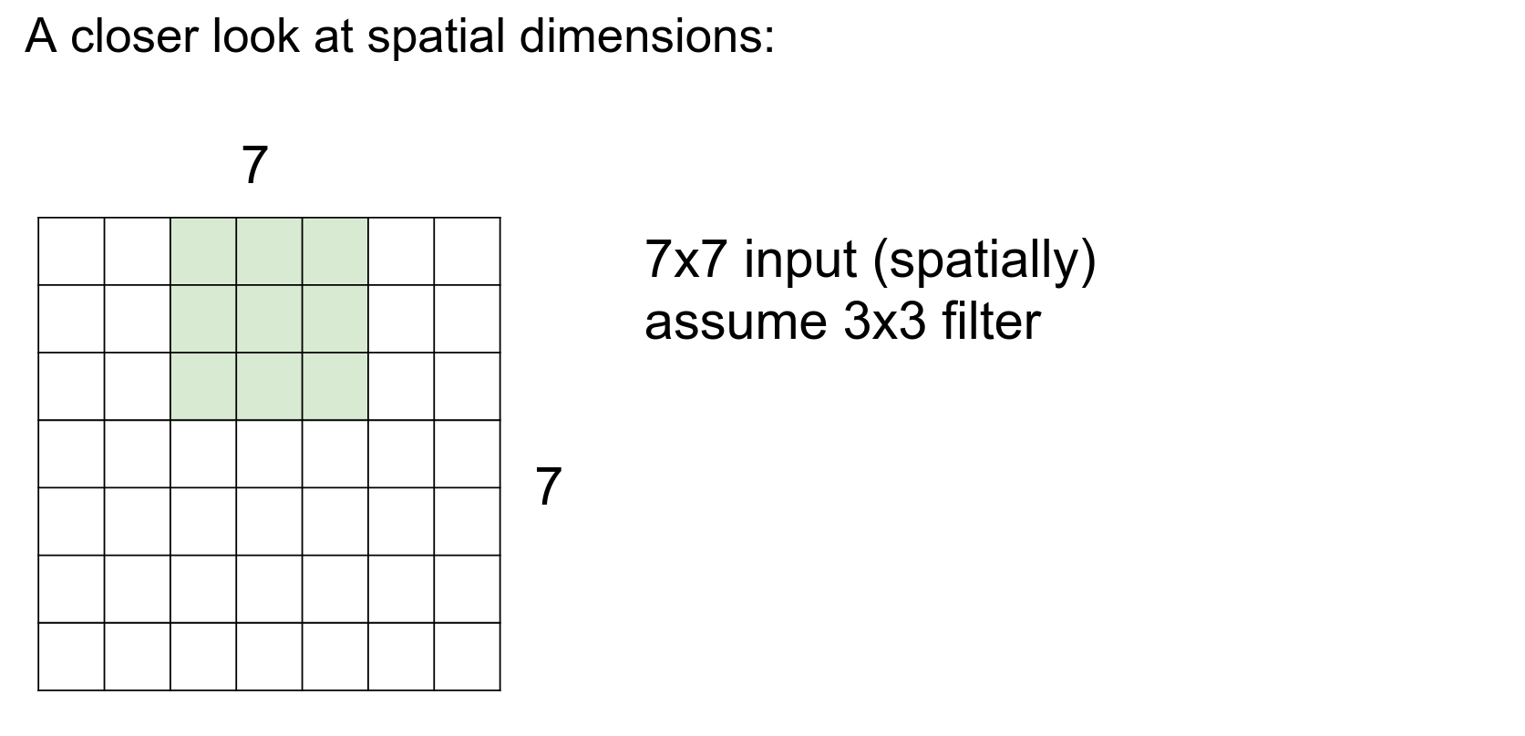
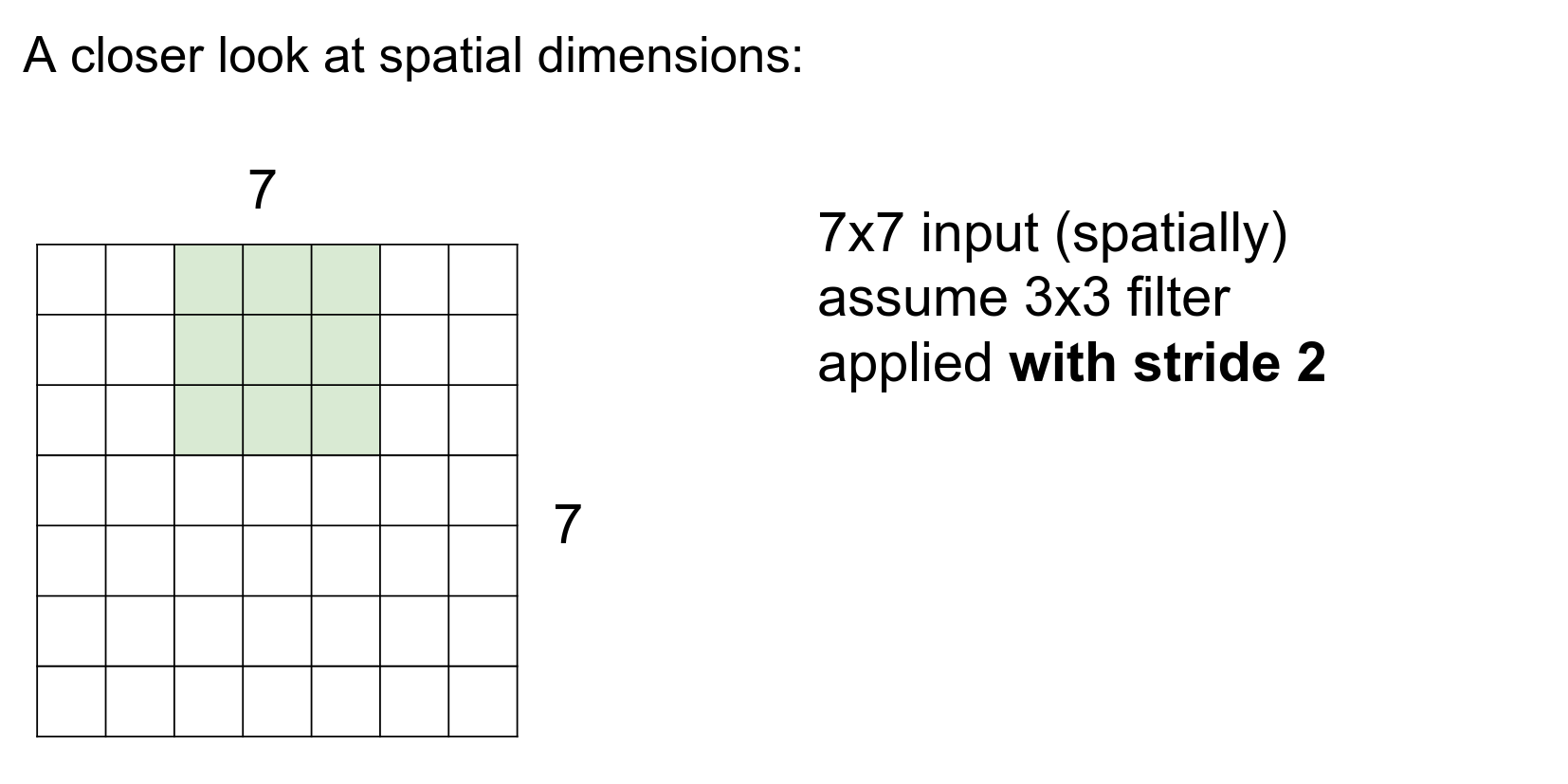
We are only concerned about spatial dimensions at this point.

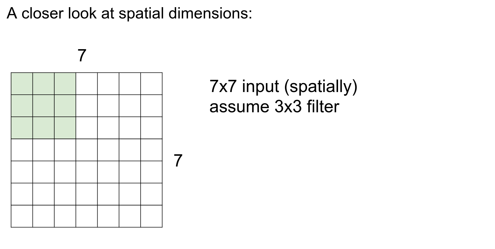
One at a time.

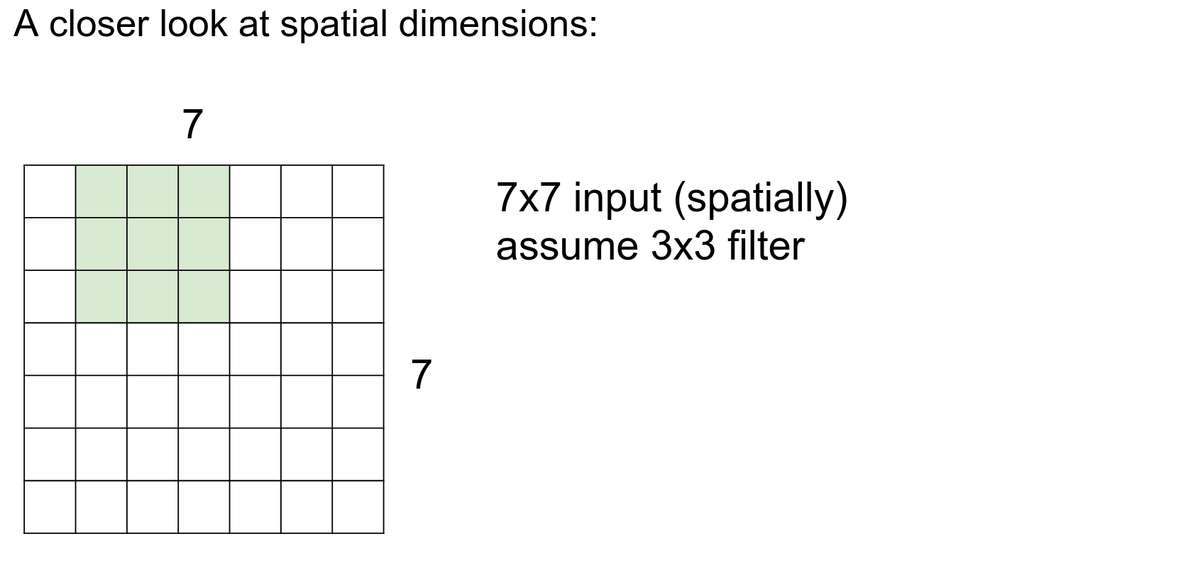
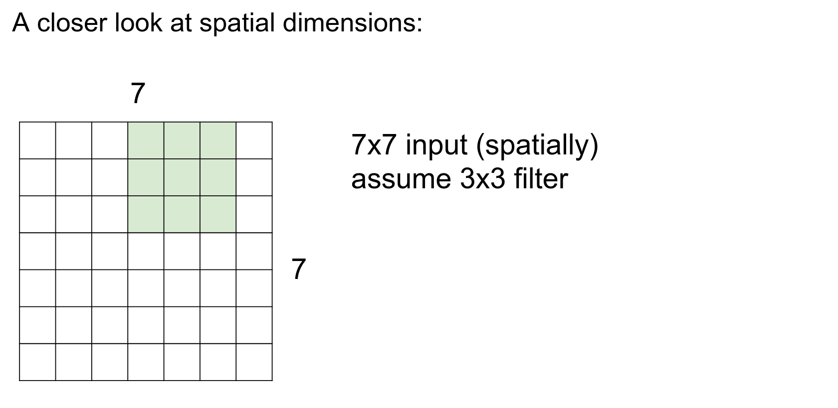
One at a time.

One at a time.

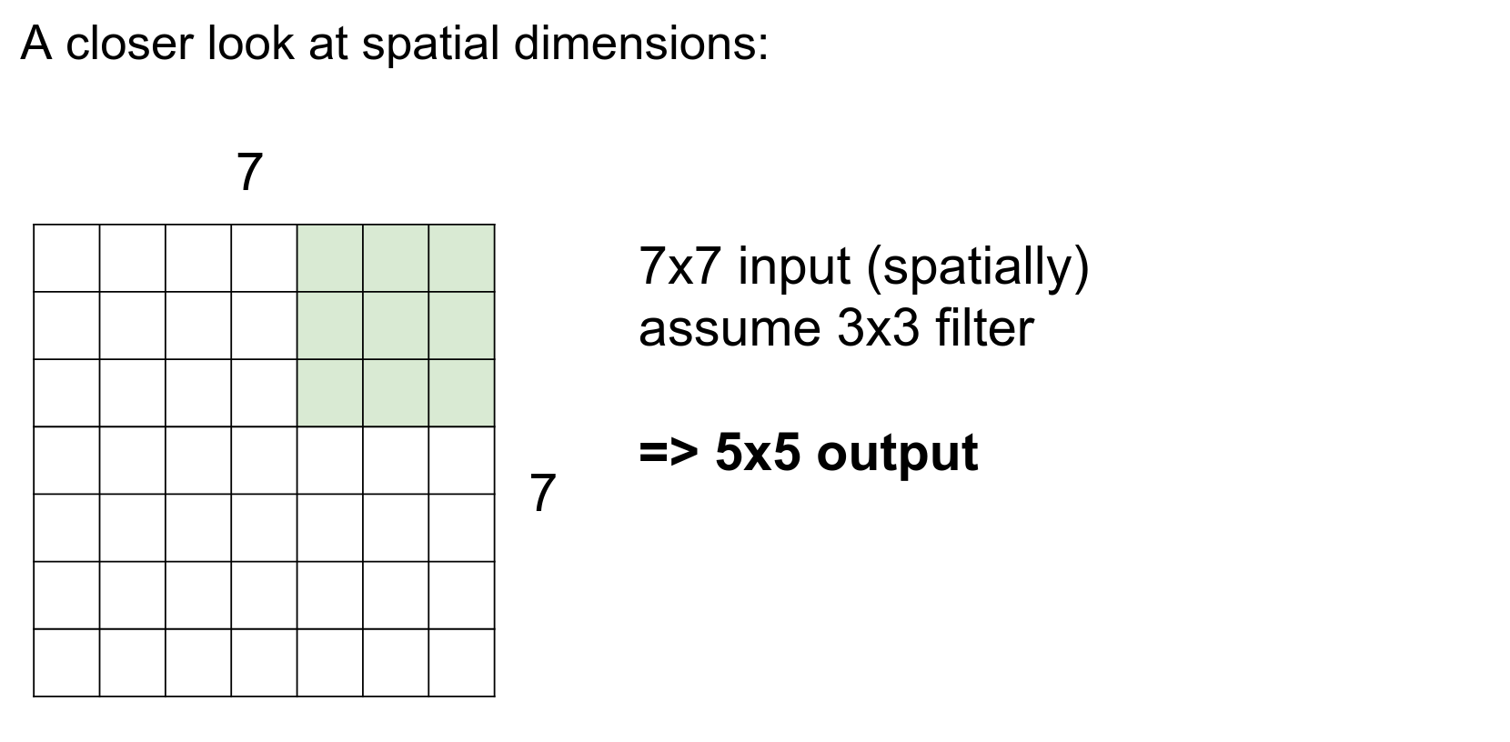
One at a time.

We can use a stride of 2, which is a hyperparameter.

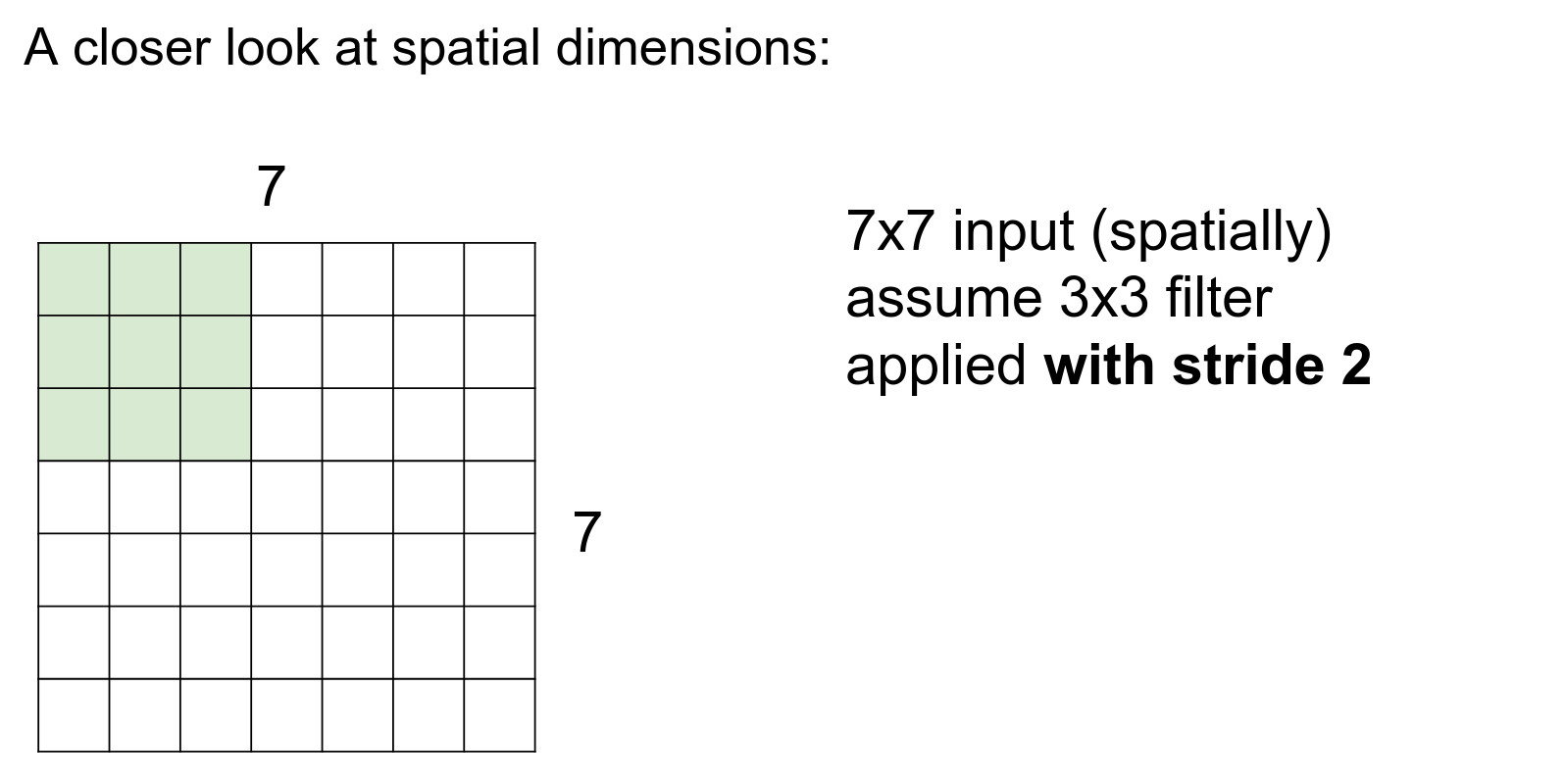
We move two steps at a time.

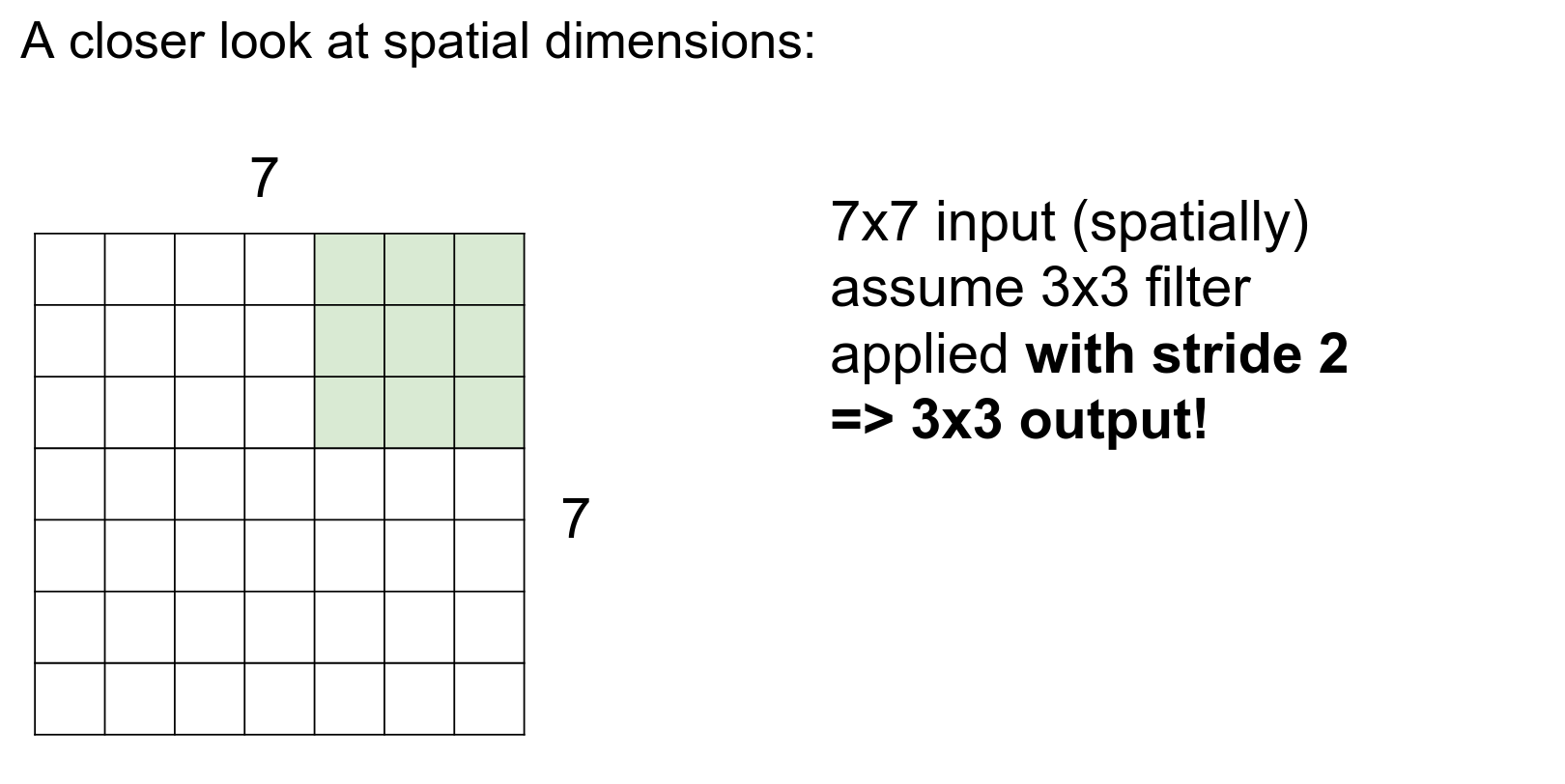
We are done in fewer steps!

Can we use a stride of 3?

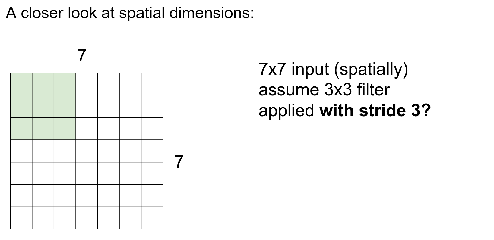
No, we cannot.

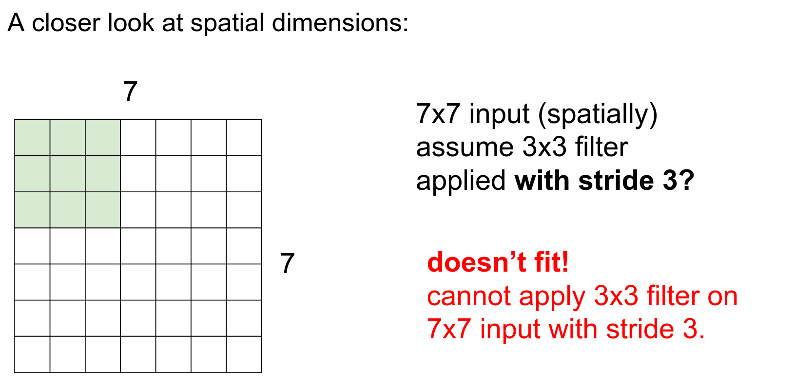
This simple formula gives you possible selections. The result should always be an integer.

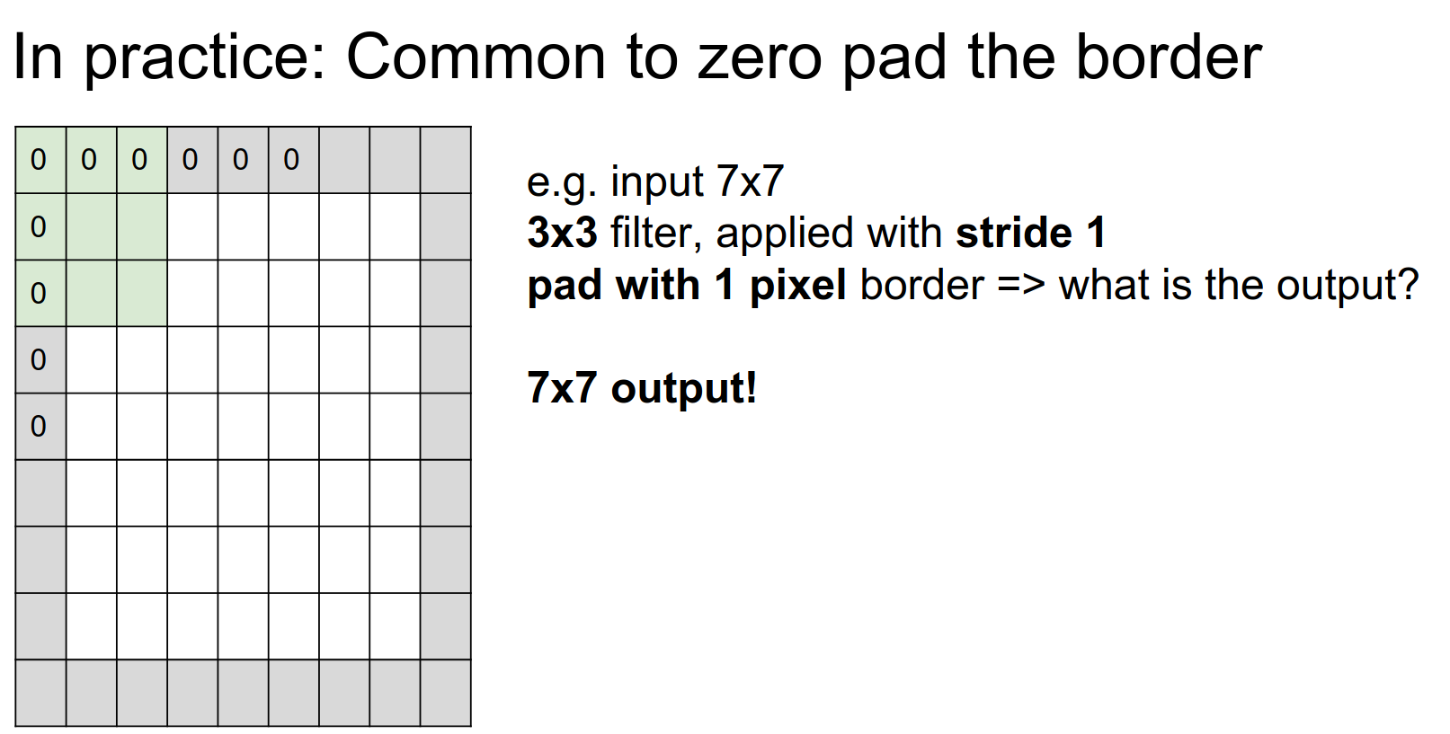
We can pad! Padding is also a hyperparameter.

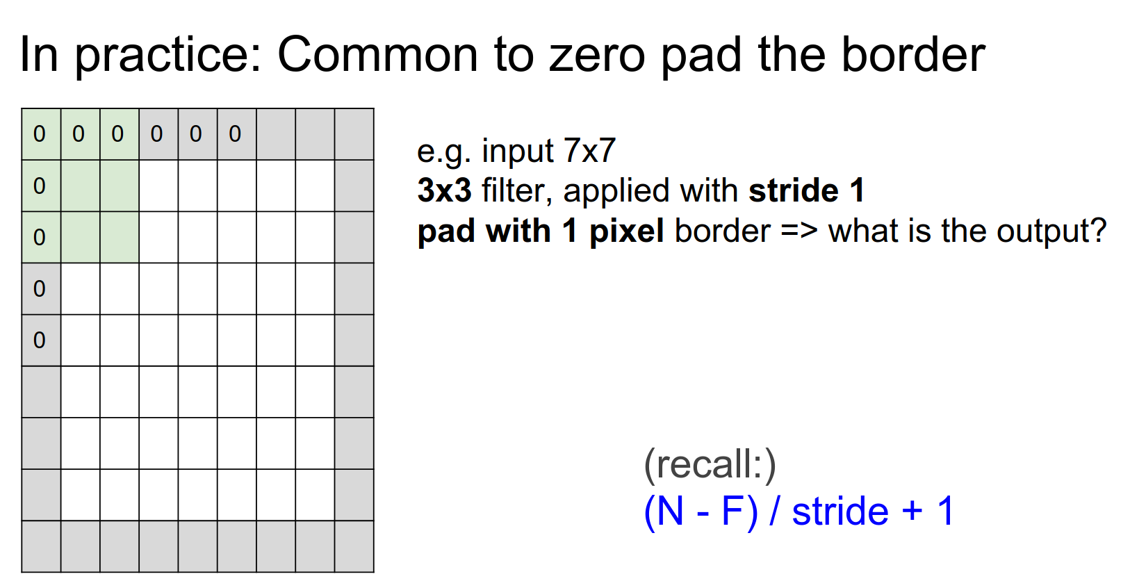
If we pad with 1, we can get an output of the same size.

Spatial Preservation

Padding Strategy

If we do not pad, the size will shrink! We do not want that, as we will have many layers.

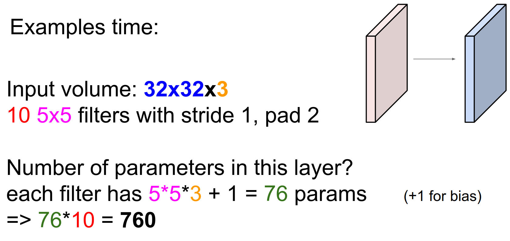
10 filters with \(5x5x3\) shape.

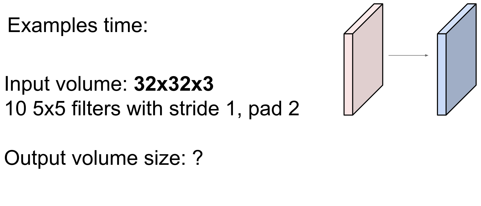
The padding is correct, so the spatial size will not change.

10 filters will generate 10 different activation maps.

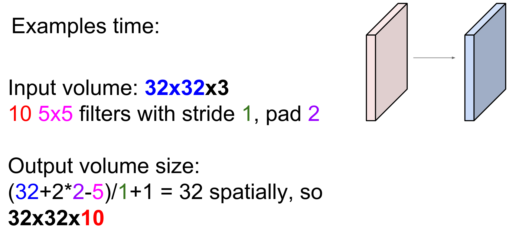
The output is shaped \(32x32x10\).

Parameter Counting

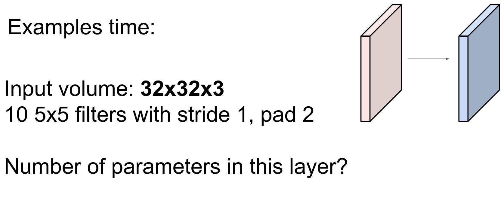
Each filter has \(5*5*3\) parameters plus a single bias. So the total is \(10 * 76 = 760\).

Here is the summary so far:

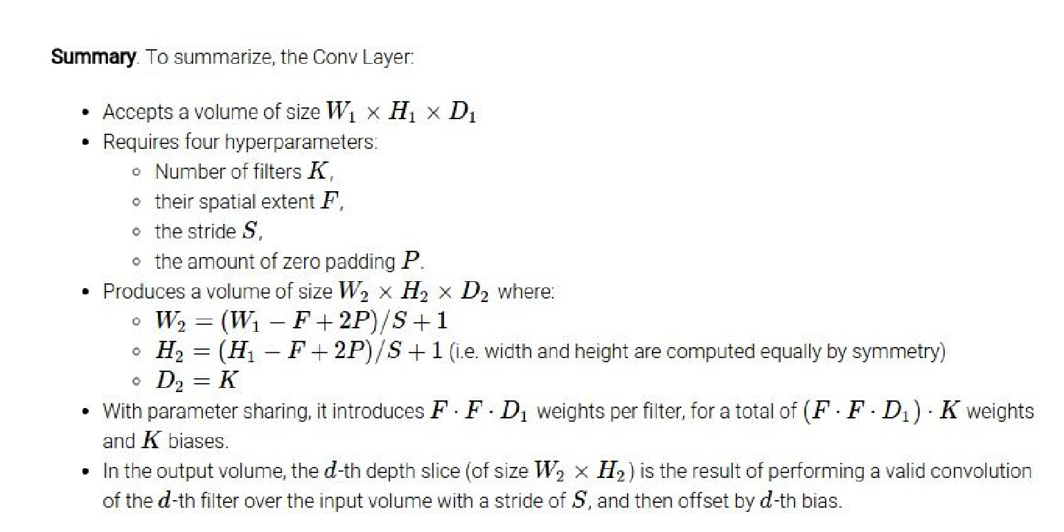
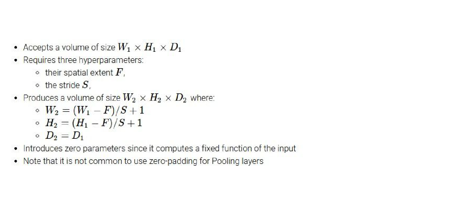
Filter Hyperparameters

• Number of filters
• The spatial extent of the filters - \(F\)
• The stride - \(S\)
• The amount of zero padding - \(P\)

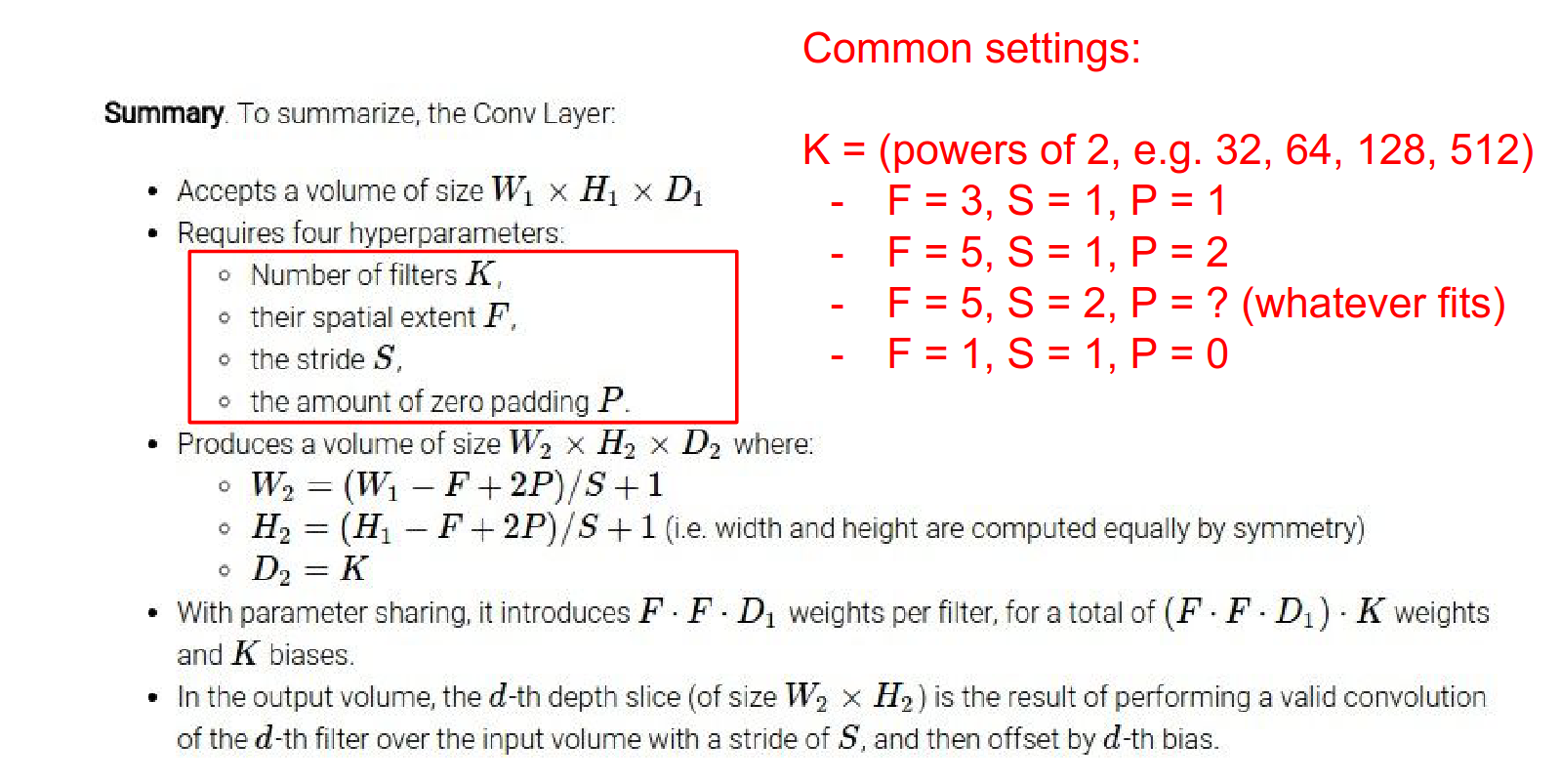
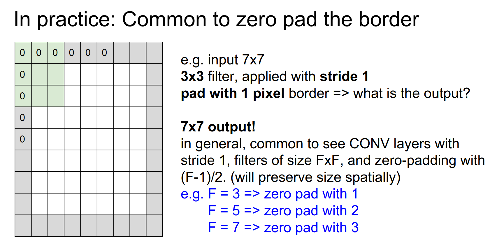
We can compute the size of the activation output with the formula. The depth will be the number of filters \(K\). \(F\) is usually odd.

The total number of parameters will depend on input depth, filter size, and bias.

\(K\) is usually chosen as a power of 2 for computational reasons. Some libraries use special subroutines when they see powers of 2.

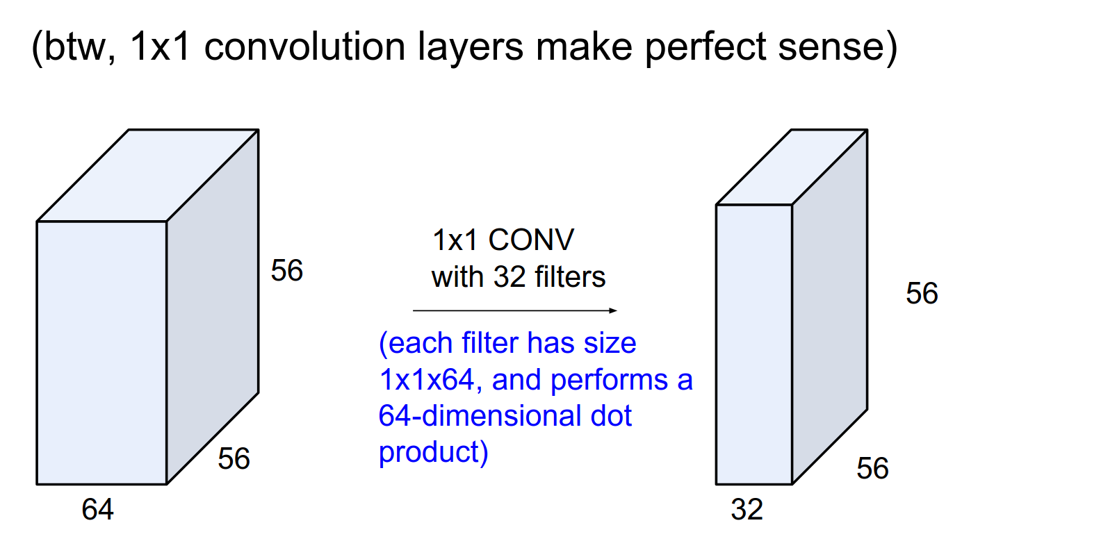
We can use \(1x1\) convolutions. You are still doing a lot of computation; you are just not merging information spatially.

Zero Padding Rationale

Non-Square Inputs

We will see how to work with non-rectangular images later.

Terminology

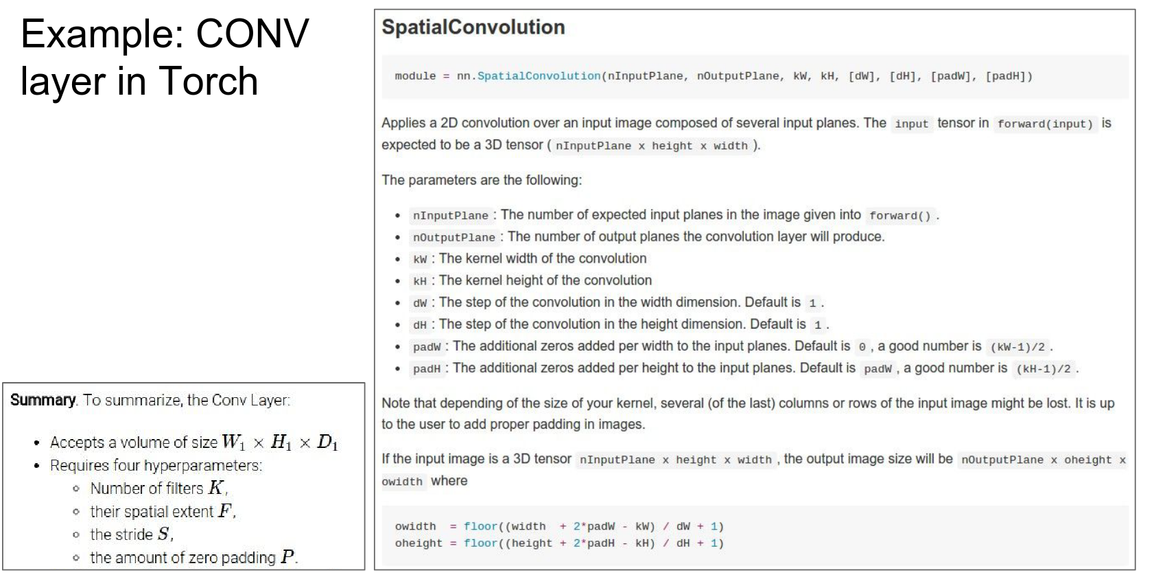
The API of SpatialConvolution in Torch:

• nInputPlane: The depth of the input layer.

• nOutputPlane: How many filters you have.

• kW, kH: Kernel width and height.

• dW, dH: Step size (stride).

• padW, padH: The padding you want.

This is referring to Lua Torch (Torch7), which was the predecessor to the modern PyTorch, with this Conv2d class here.

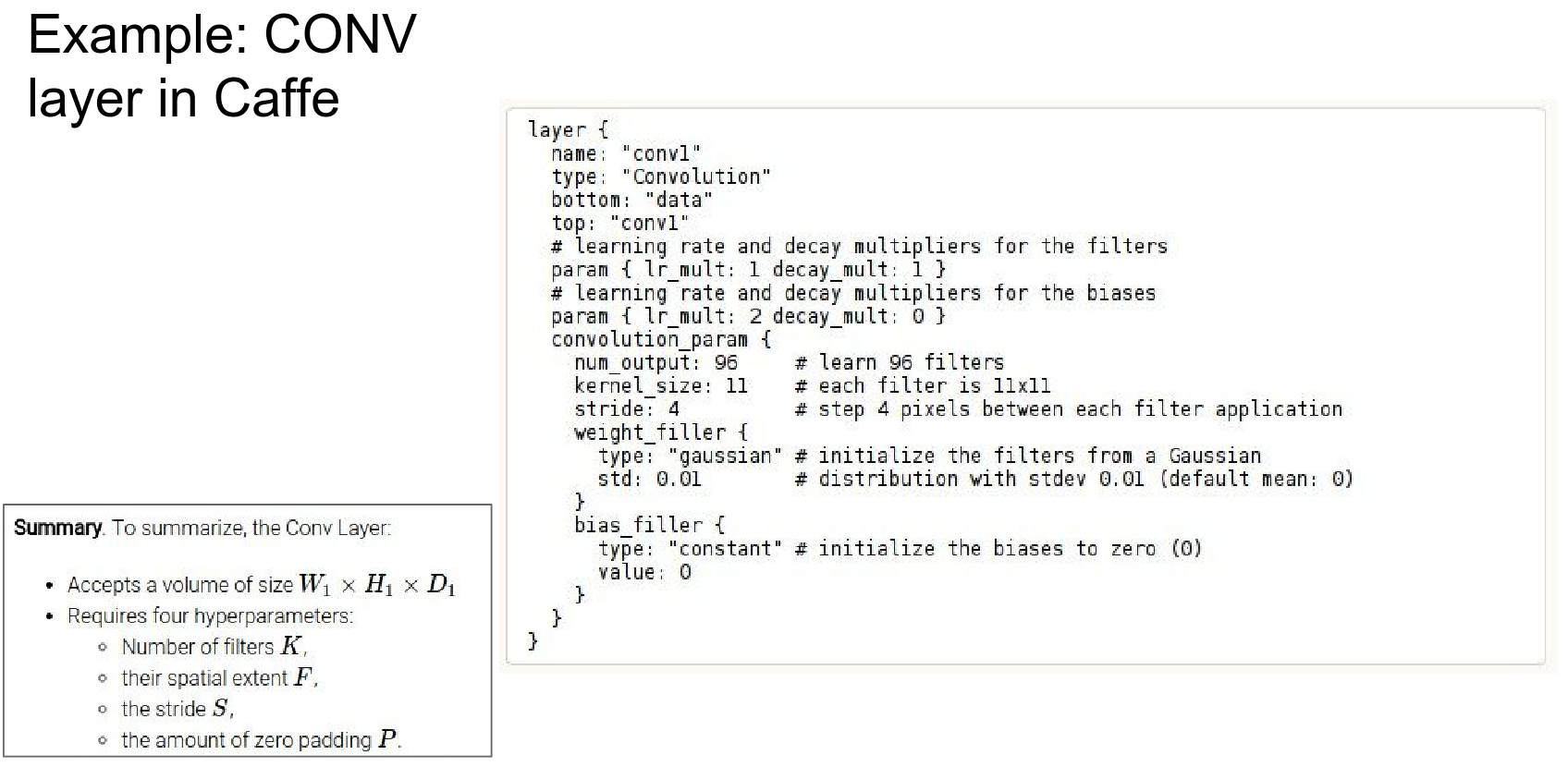
It is the same in Caffe.

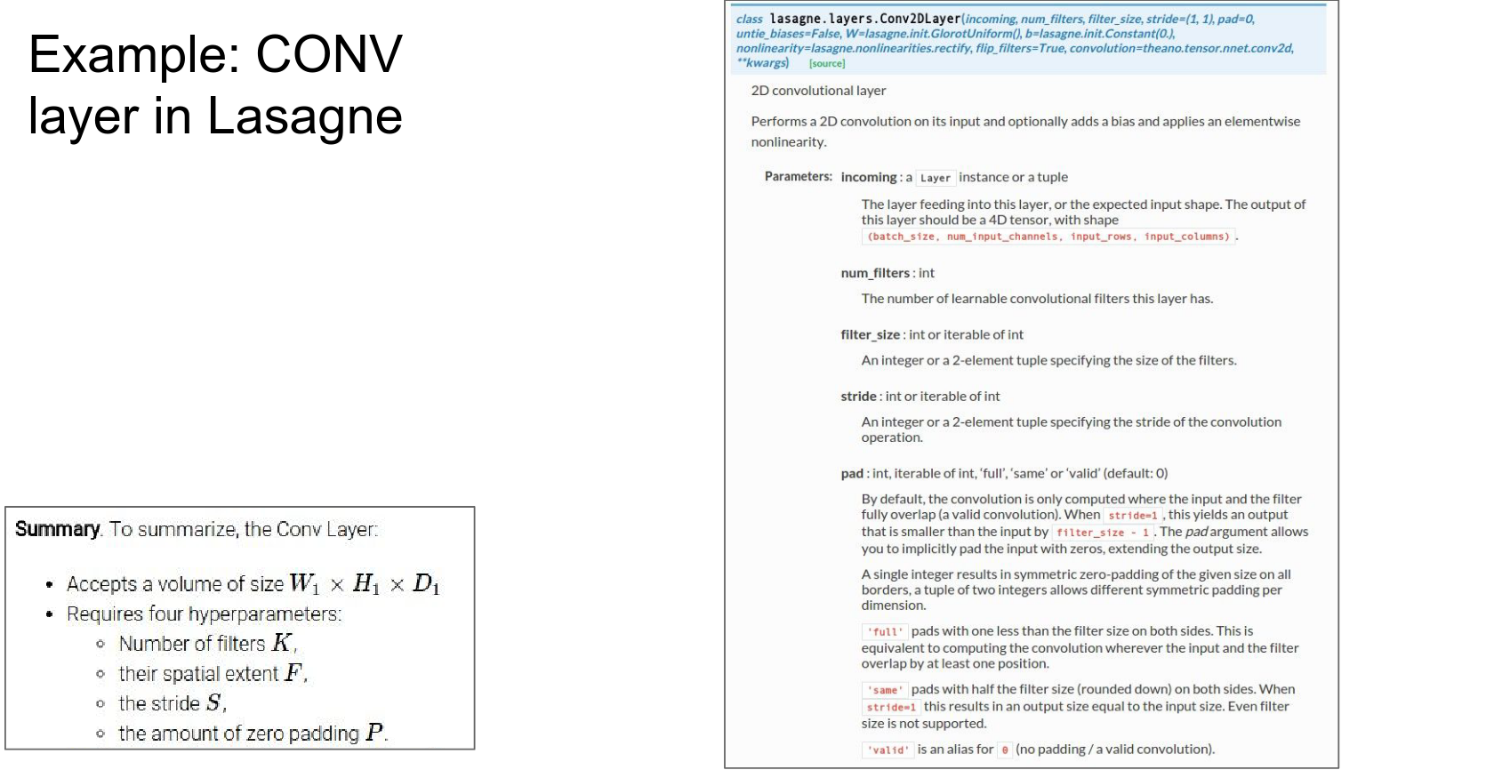
It is the same in Lasagne.

Biological Perspective

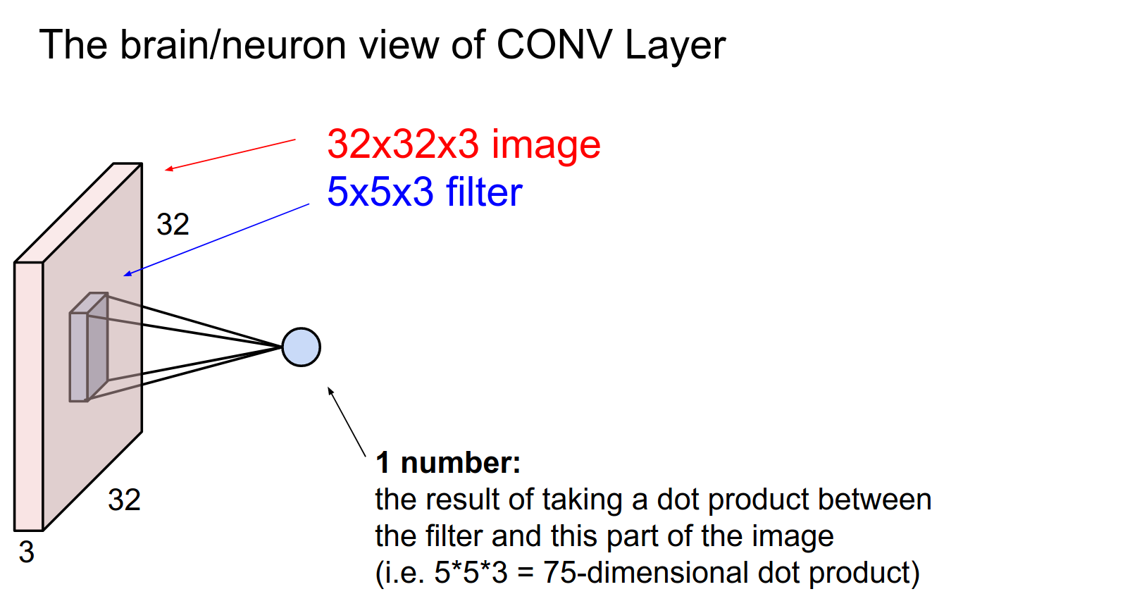
With this filter, we end up with one number in a convolution.

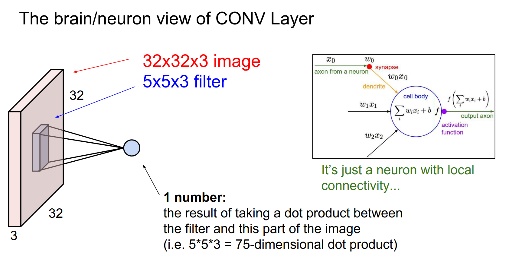
The output of the filter at this position is just a neuron fixed in space, looking at a small part of the input, computing \(w^T x + b\).

It has no connections to other parts of the image, hence local connectivity.

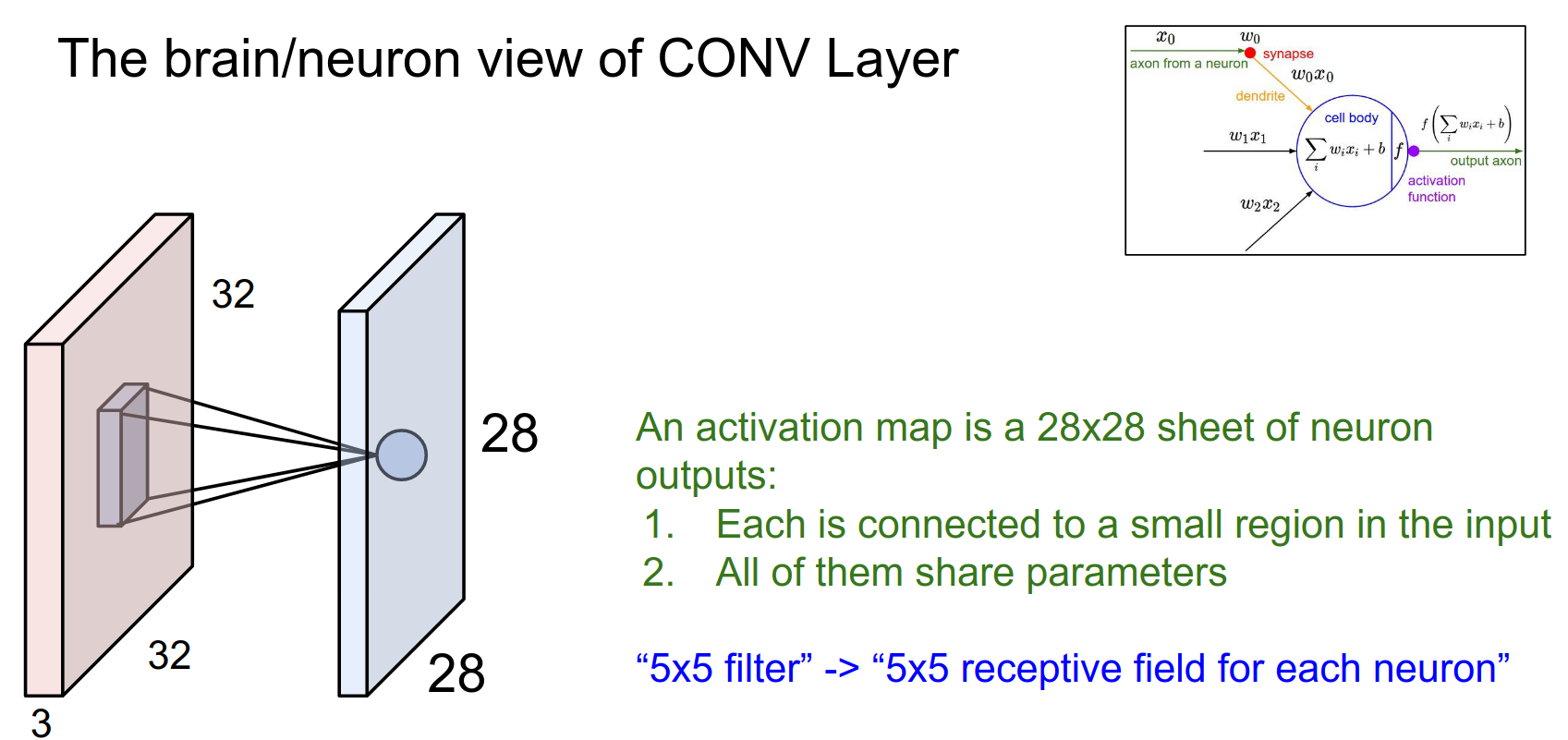
We sometimes refer to the neuron's receptive field as the size of the filter (the region of the input the filter is looking at).

In a single activation map (28x28 grid), these neurons share parameters (because one filter computes all the outputs), so all the neurons have the same weights \(w\).

Weight Sharing

We have several filters, so spatially they share weights, but across depth, these are all different neurons.

A nice advantage of both local connectivity and spatial parameter sharing is that it basically controls the capacity of the model.

It makes sense that neurons would want to compute similar things. For example, if they are looking for edges, a vertical edge in the middle of an image is just as useful anywhere else spatially.

It makes sense to share those parameters spatially as a way of controlling overfitting.

We have covered Conv and ReLU layers.

Pooling Layer

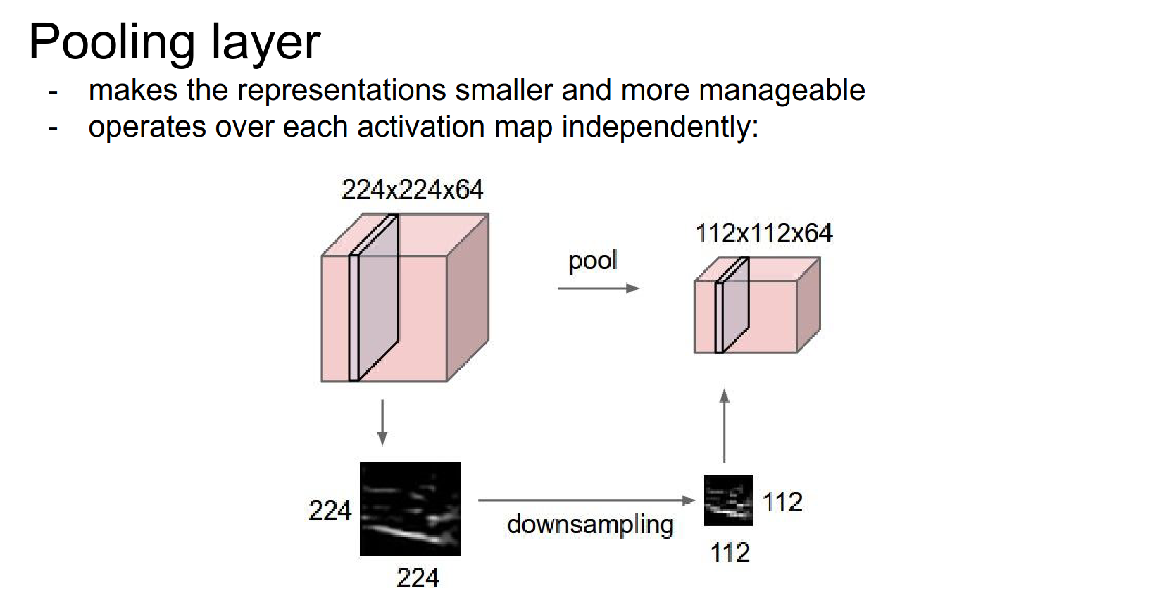
The Conv layer usually preserves the spatial size (with padding).

The spatial shrinking is done by pooling.

Motivation

The most common method is max pooling.

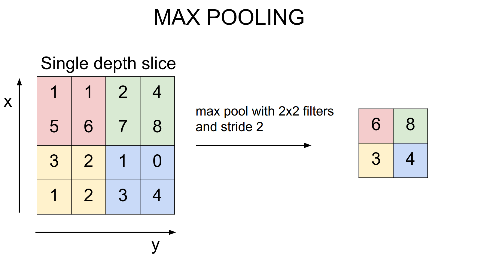
It reduces the size by half on all activation maps. Average pooling does not work as well.

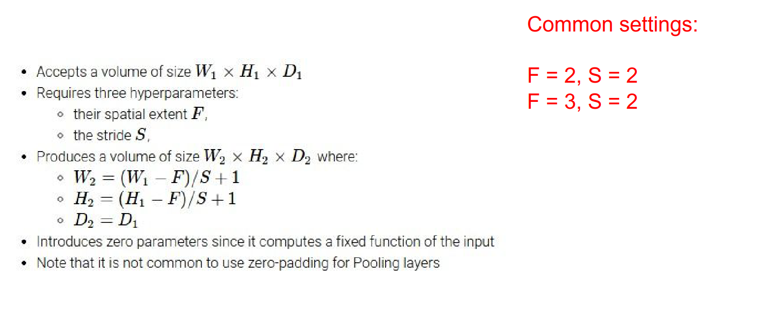
We need to know the filter size and stride. \(2x2\) with stride \(2\) is common.

The depth of the volume does not change.

Fully Connected Layer

With 3 pooling layers (\(2x2\), stride 2), we go from 32 -> 16 -> 8 -> 4.

At the end, we have a \(4x4x10\) volume of activations after the last pooling.

That goes into the Fully Connected layer.

Demo

Website here. It achieves 80% accuracy for CIFAR-10 in JavaScript!

It uses 6 or 7 nested loops. The V8 engine in Chrome is good, so JS is fast.

All running in the browser.

---

Stacking Layers

Why is that we are stacking layers? 🤔

Because we want to do dot products, and we can backpropagate through them efficiently.

Batch Dimensions

If you are working with image batches, all the volume between Convnet's are 4D arrays. If single image, 3D arrays.

Visualization

Intermediate filters are not properly visualized. Yann LeCun did what the neurons are responding to.

Pooling Rationale

When you do pooling, you throw away some spatial information because you want to eventually get the scores out.

Boundary Effects

Because of padding, the statistics of border is different than center, we do not worry about it.

Backpropagation Compatibility

Anything you can back propagate through, you can put in a ConvNet / Neural Net.

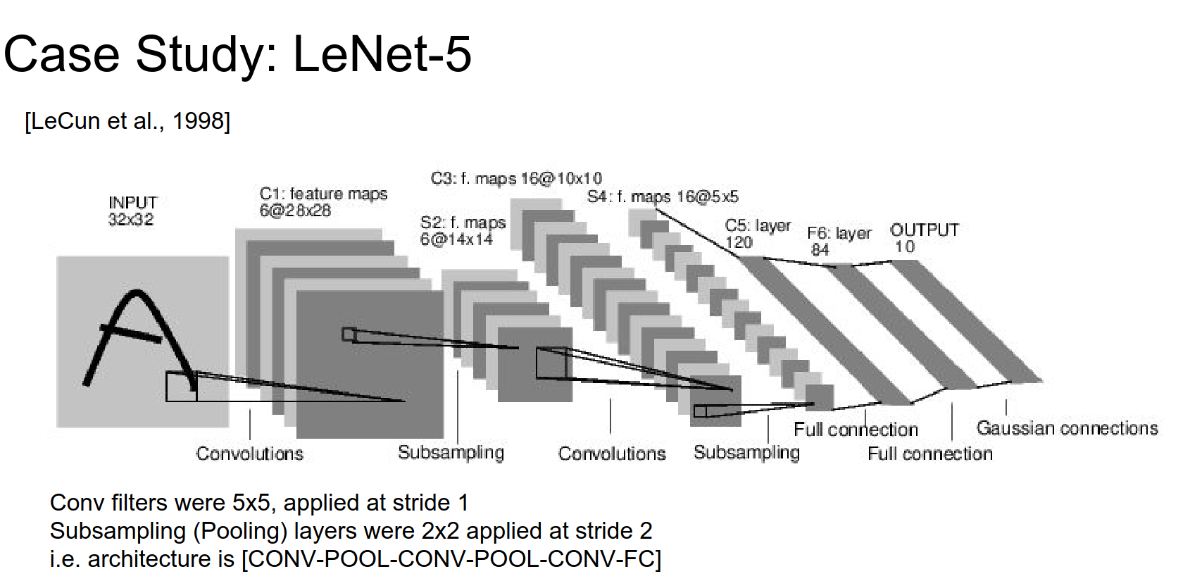
Case Studies

LeNet-5

Figure from the paper. 6 filters, all \(5x5\), with sub-sampling (max pooling).

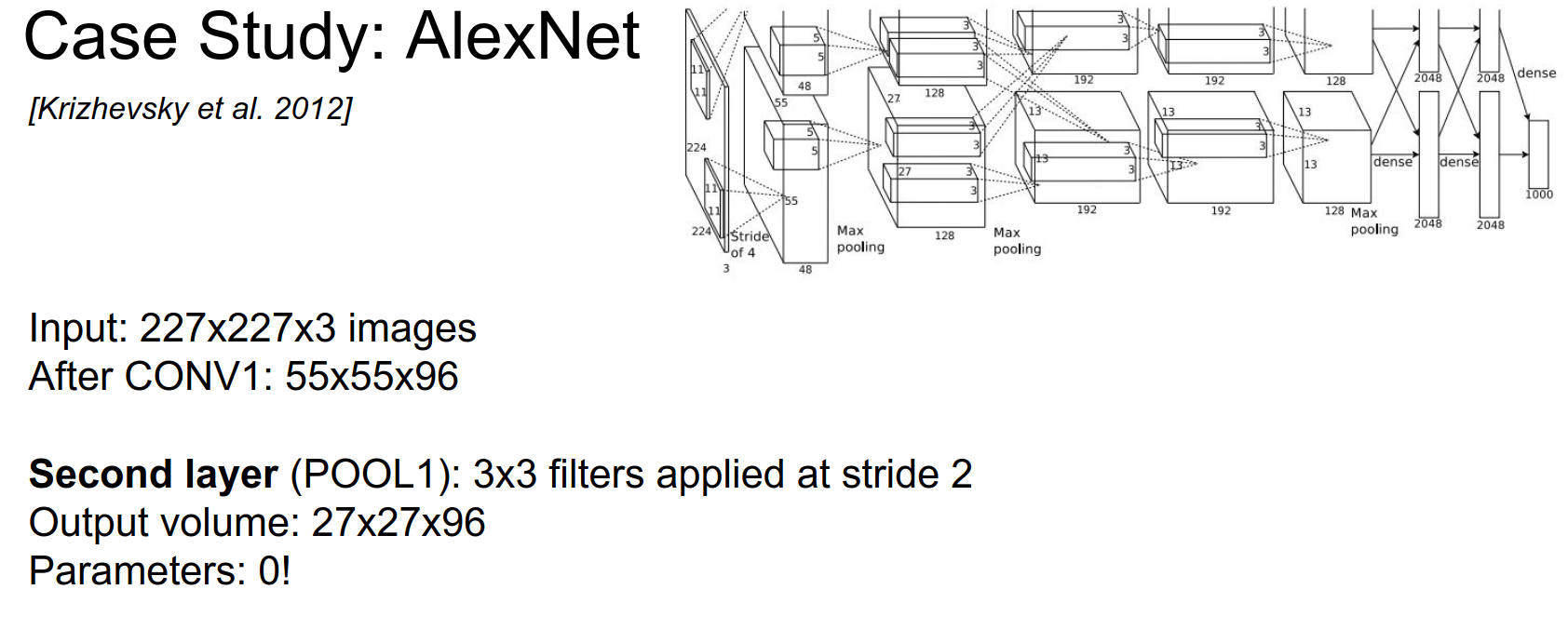
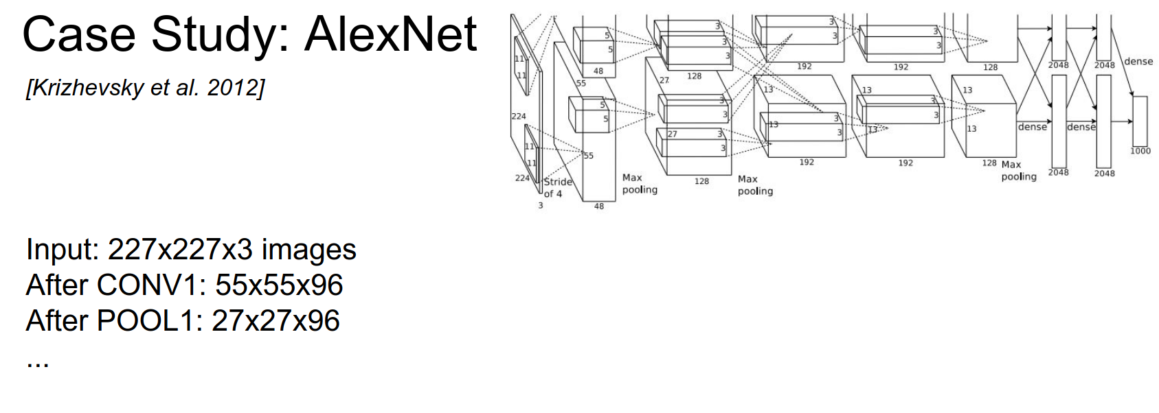
AlexNet

It won the ImageNet challenge. 60 Million Parameters.

The input is large.

Two separate streams? Alex had to split the convolutions onto 2 separate GPUs.

Let's imagine if it had a single stream.

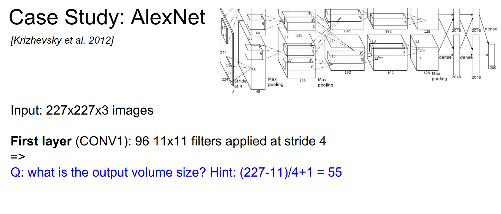
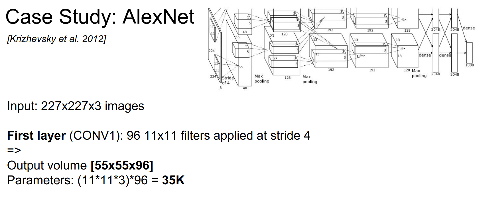
The output volume will be: \(55x55x96\), because we have 96 kernels/filters.

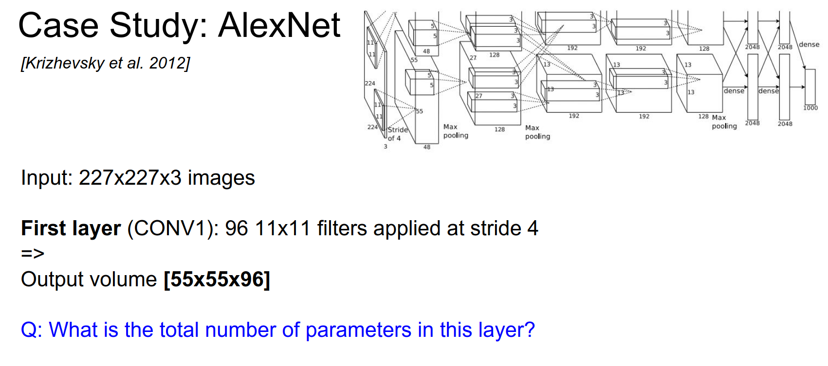
Total parameters: every filter is \(11x11x3\) x 96 roughly.

We are not even sure what Alex did. 😅

The input image is \(224x224\), but for the math to add up, the input should be \(227x227\).

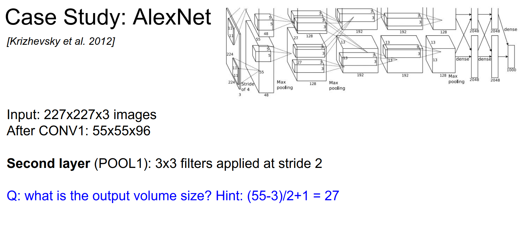
After pooling? Half of the spatial size, so \(27x27x96\).

How many parameters are in the pooling layer?

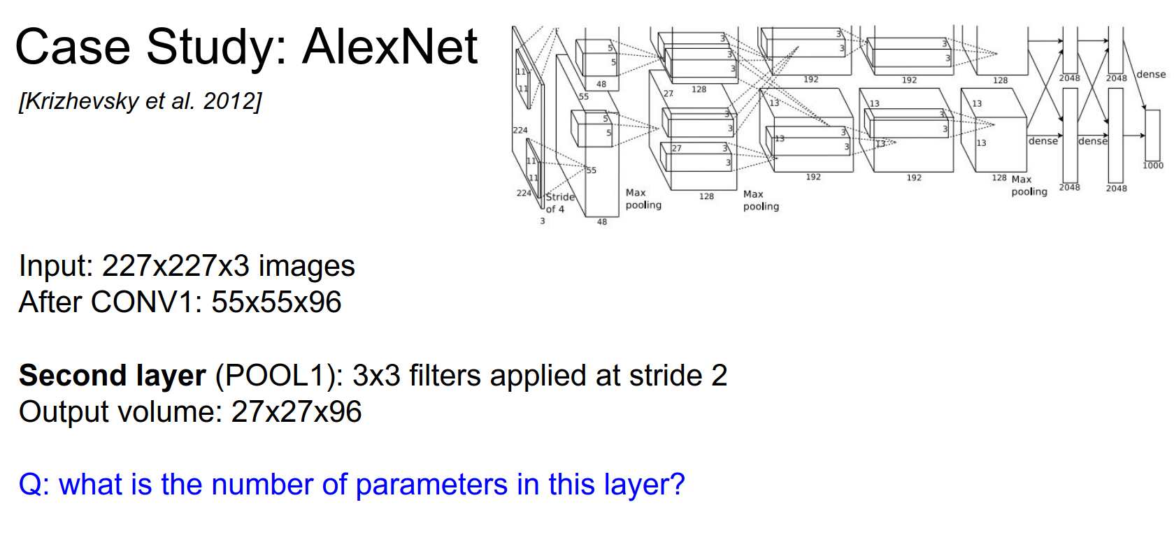
0 - only Conv layers have parameters.

Summary:

Full architecture:

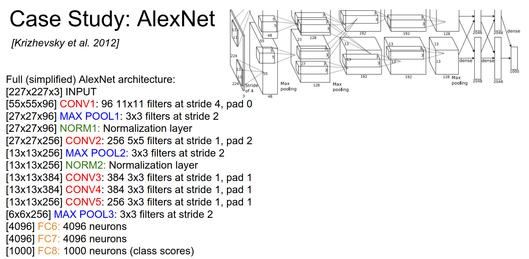
This is a classic sandwich. Sometimes filter sizes change. We backpropagate through all of this.

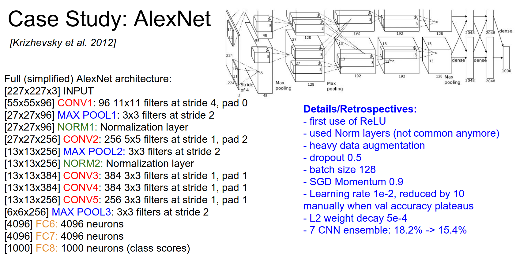
First use of ReLU, used normalization layers (not used anymore), used dropout only on the last fully connected layers, and an ensemble of 7 models.

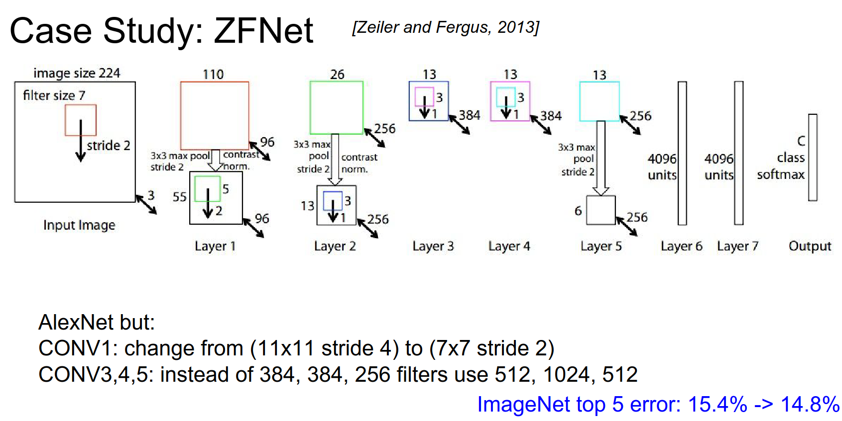
ZFNet

Built on top of AlexNet.

\(11x11\) stride 4 was too drastic, so they changed to \(7x7\) filters.

They used more filters in Conv 3, 4, and 5.

The error became 14.8%. The author of this paper founded a company called Clarifai and reported 11% error.

Here is the company about.

Founded in 2013 by Matthew Zeiler, Ph.D., a foremost expert in machine learning, Clarifai has been a market leader since winning the top five places in image classification at the ImageNet 2013 competition.

Top-5 Error

There are 1000 classes, and we give the classifier 5 chances to guess. 😌

VGGNet

140 Million Parameters. They have different types of architectures. They decided to use a single set of filters. The question is:

Layer Count

Turns out, 16 layers performed the best. They dropped the error to 7.3%.

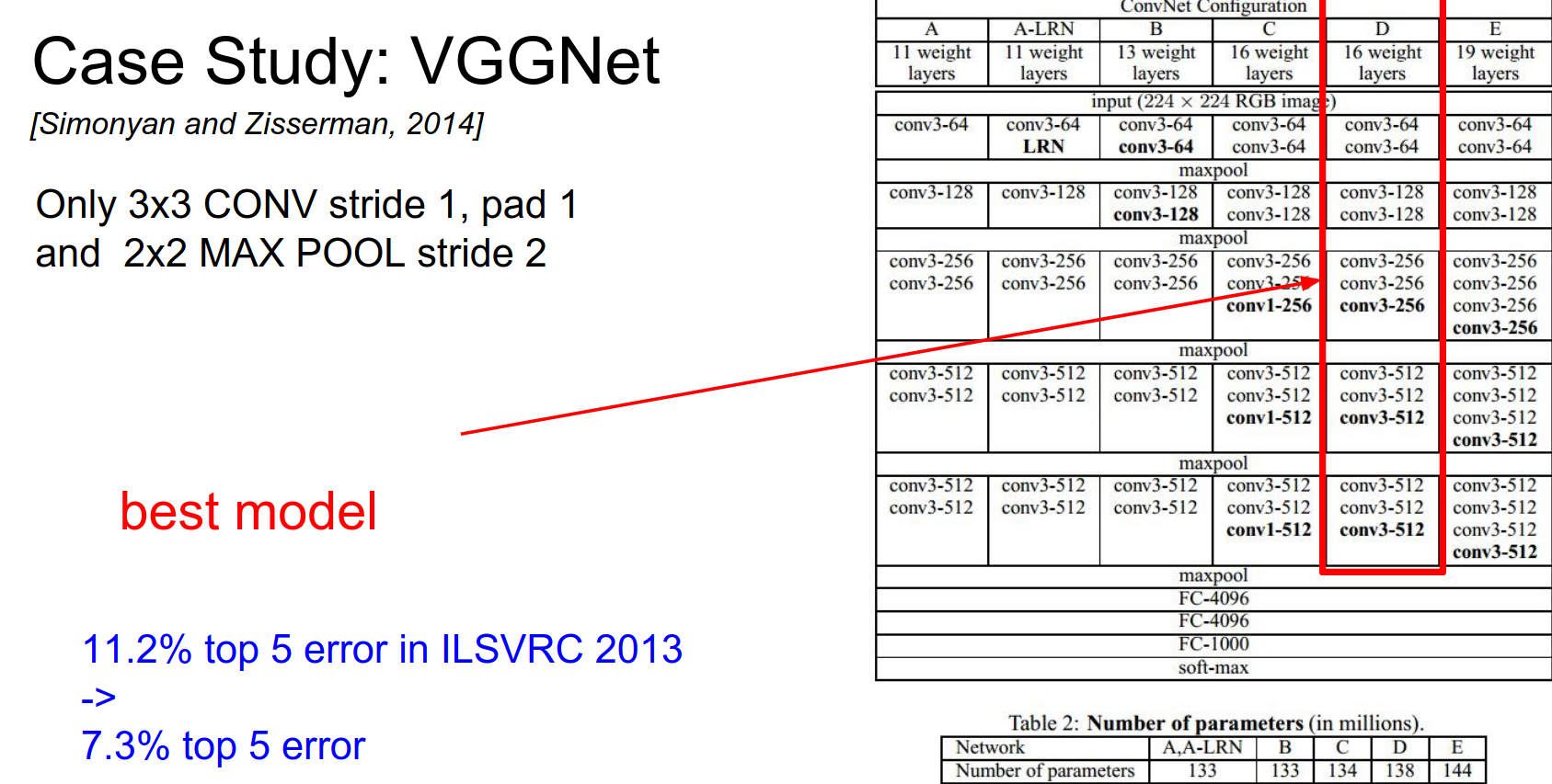
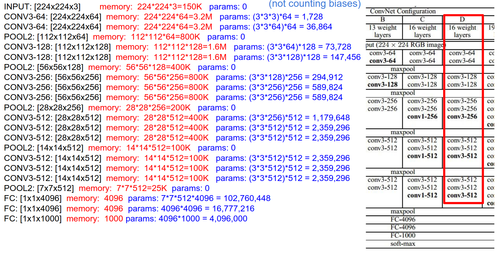
This is the full architecture:

Spatial Reduction

Spatially the volumes get smaller, number of filters are increasing

Memory Usage

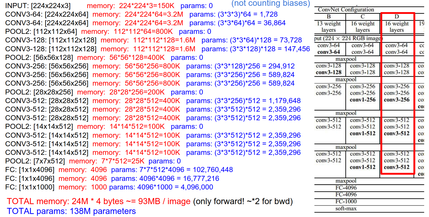
If we add up all the numbers, it's 24M. If we use float32, that's 93 MB of memory for intermediate activation volumes per image.

That is maintained in memory because we need it for backpropagation.

Just to represent 1 image, it takes 93 MB of RAM ONLY for the FORWARD pass. For the backward pass, we also need the gradients, so we end up with a 200 MB footprint.

Parameter Count

Most memory is in early Conv layers; most parameters are in late FC layers.

We found that these huge Fully Connected layers are not necessary.

Average Pooling

Instead of FC on \(7x7x512\), you can average on \(7x7\) and make it a single \(1x1x512\), which works just as well.

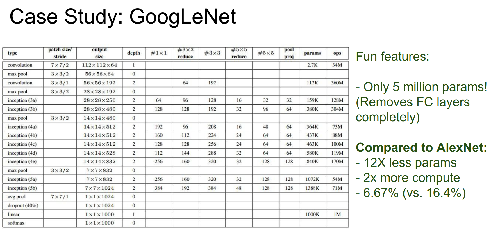
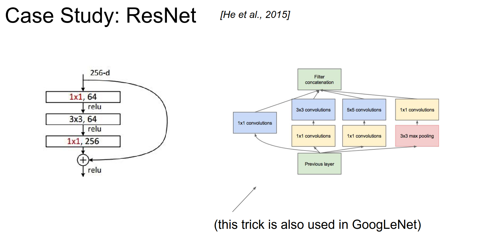
GoogleNet

The key innovation here was the Inception module. Instead of using direct convolutions, they used inception modules.

A sequence of inception modules makes up GoogleNet. You can read the paper.

It won the 2014 challenge with 6.7% error.

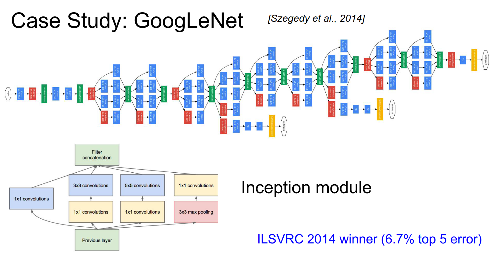
At the very end, they had \(7x7x1024\) and they did an average pool! That means much fewer parameters!

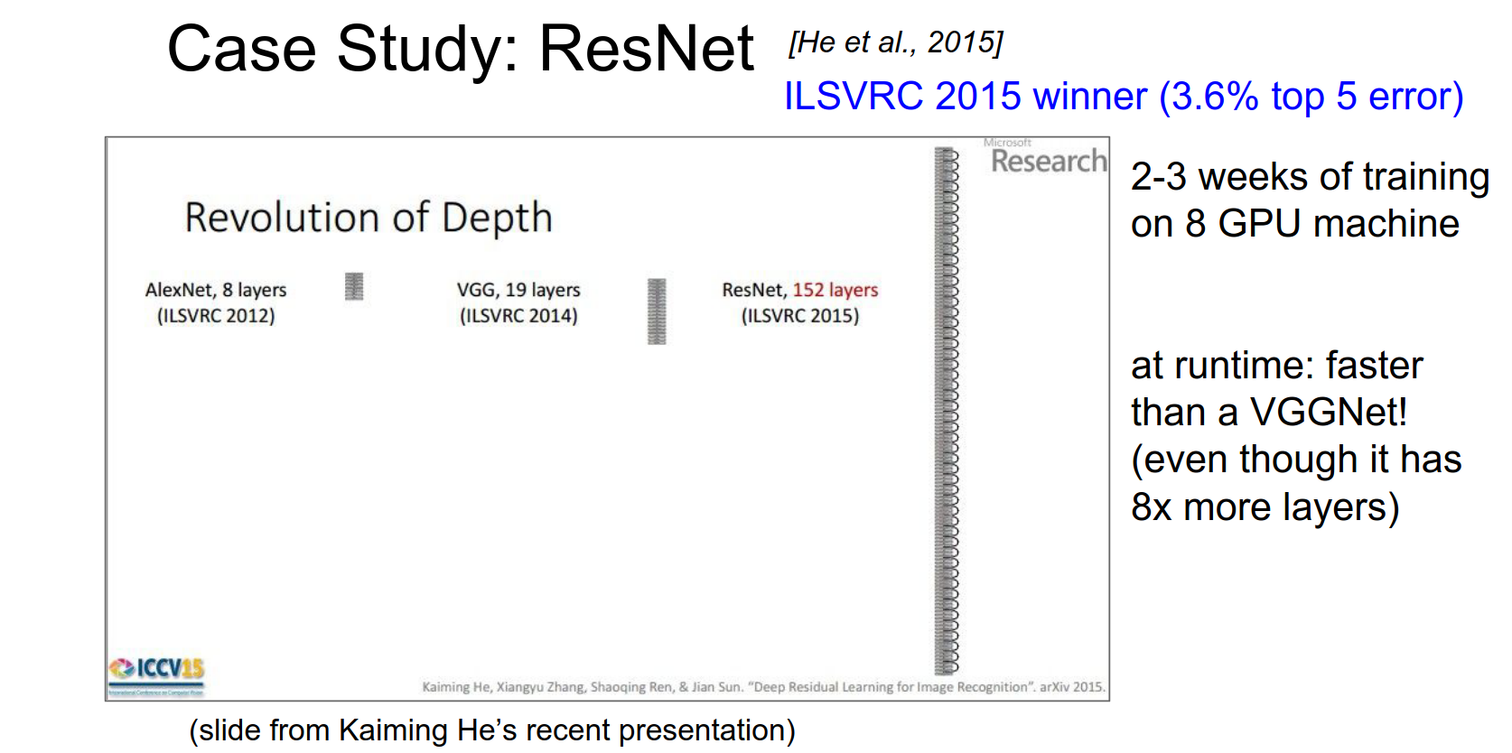
ResNet

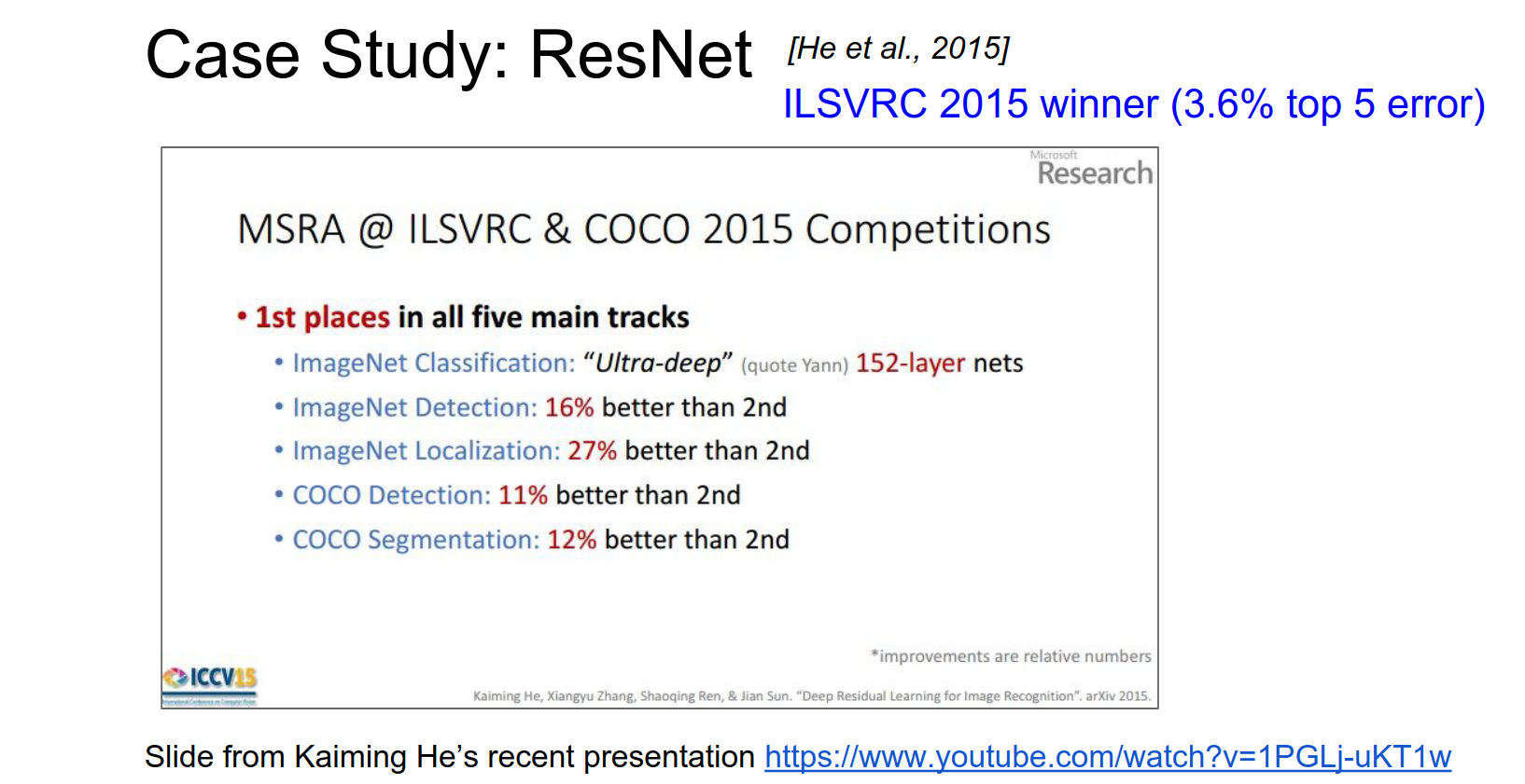
Here is what the history looks like.

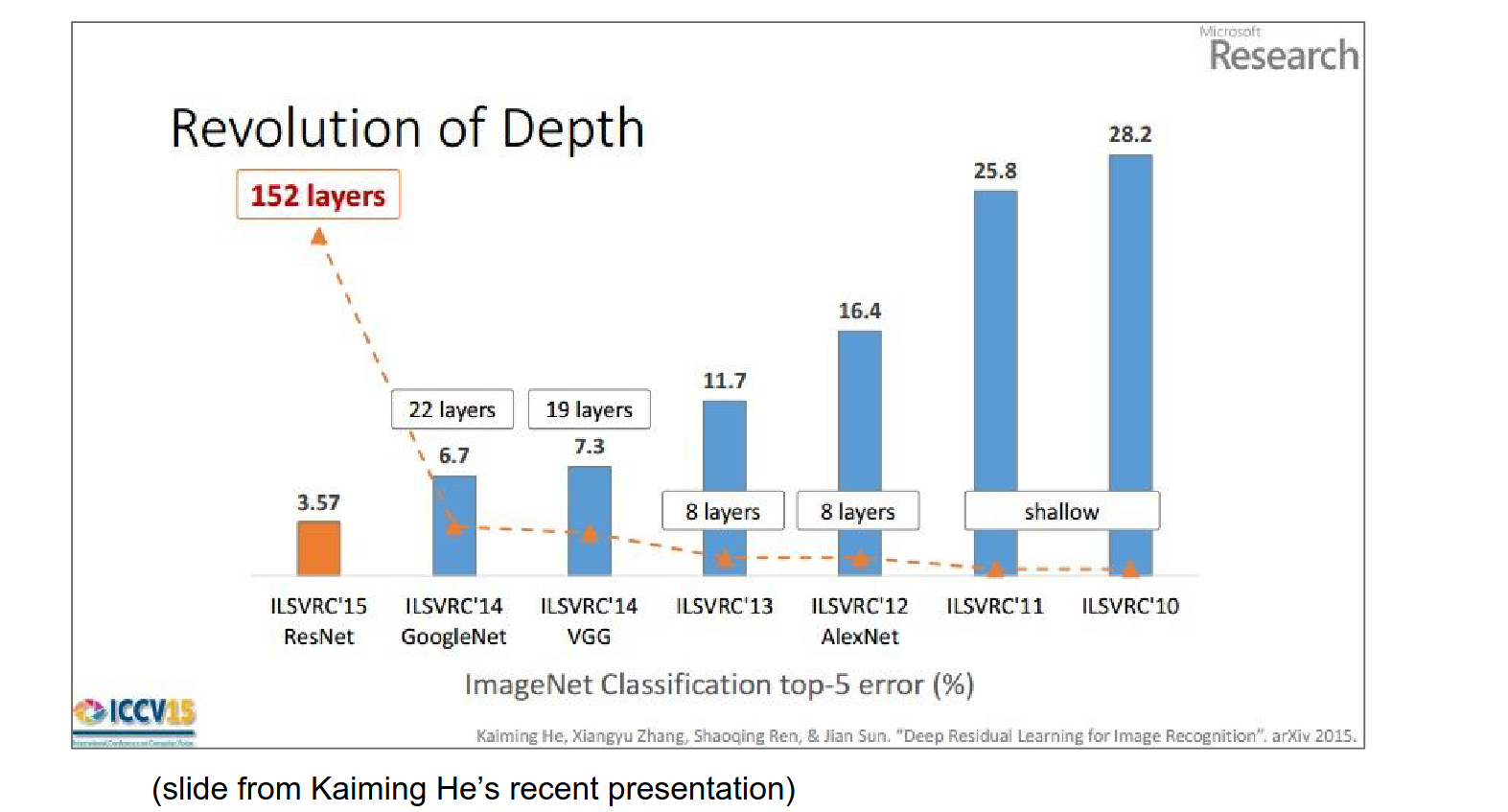
More layers. You have to be careful how you increase the number of layers.

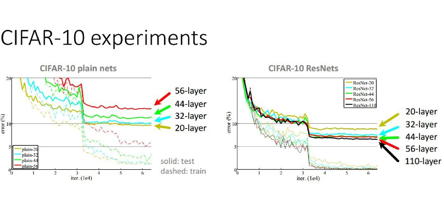
Plain vs ResNets

A 56-layer network performs worse than a 44-layer network. Why?

In ResNets, increasing the number of layers will always result in better results.

Runtime Performance

At Runtime, it is actually faster than a VGGnet - how ?

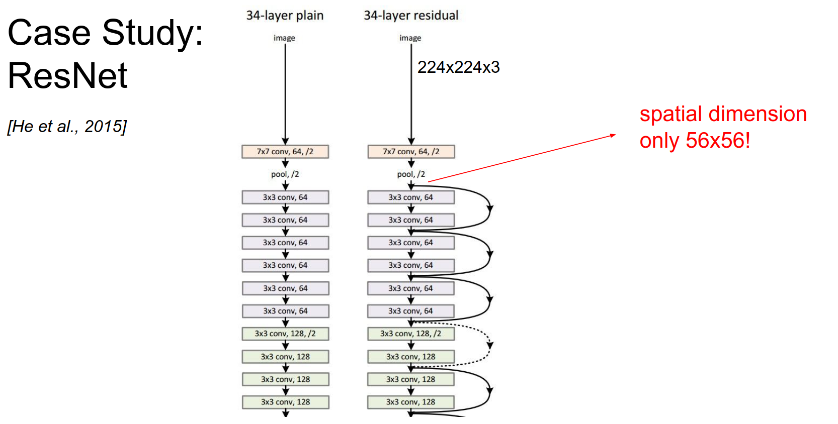
This is a plain net below:

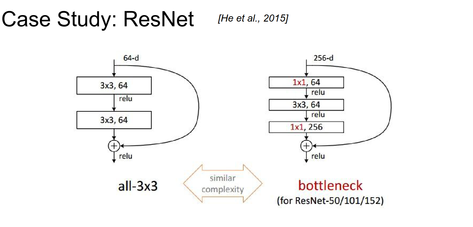
We will have skip connections.

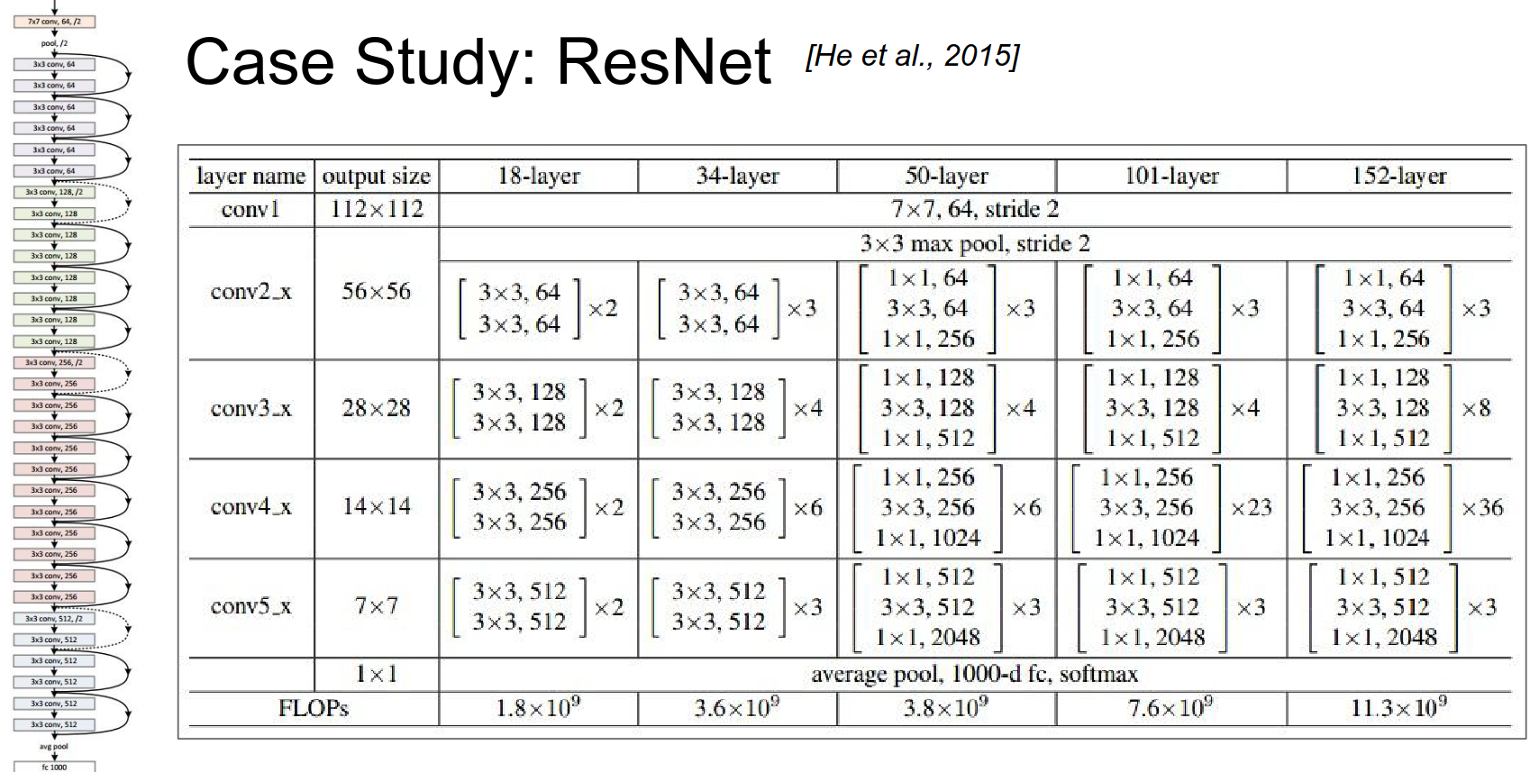
You take a \(224x224\) image, pool by a huge factor, and work spatially on \(56x56\). It's still really good.

Depth comes at the cost of spatial resolution very early on, because depth is to their advantage.

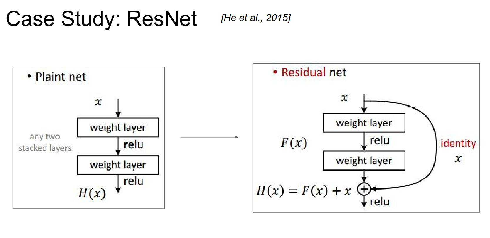
In a plain net, you have some function \(f(x)\) you are trying to compute. You transform your representation, have a weight layer, threshold it, and so on.

In a ResNet, your input flows in. But instead of computing how to transform your input into \(f(x)\), you compute what to add to your input to transform it into \(F(x)\).

You compute a delta on top of your original representation instead of a new representation right away, which would discard the original information about \(X\).

Delta Modulation Analogy

In analogy, you can think of delta modulation as encoding the difference between successive samples (input and output), somewhat akin to how the ResNet architecture focuses on learning the residual (difference) between input and output to improve learning efficiency. Both methods leverage this residual information for better representation or reconstruction.

You are computing just these deltas to these \(x\)'s.

If you think about the gradient flow in a ResNet, when a gradient comes, it performs addition (remember, addition distributes the gradient to all of its children). The gradient will flow to the top, skipping over the straight part.

You can train right away, really close to the image, to the first Conv Layer.

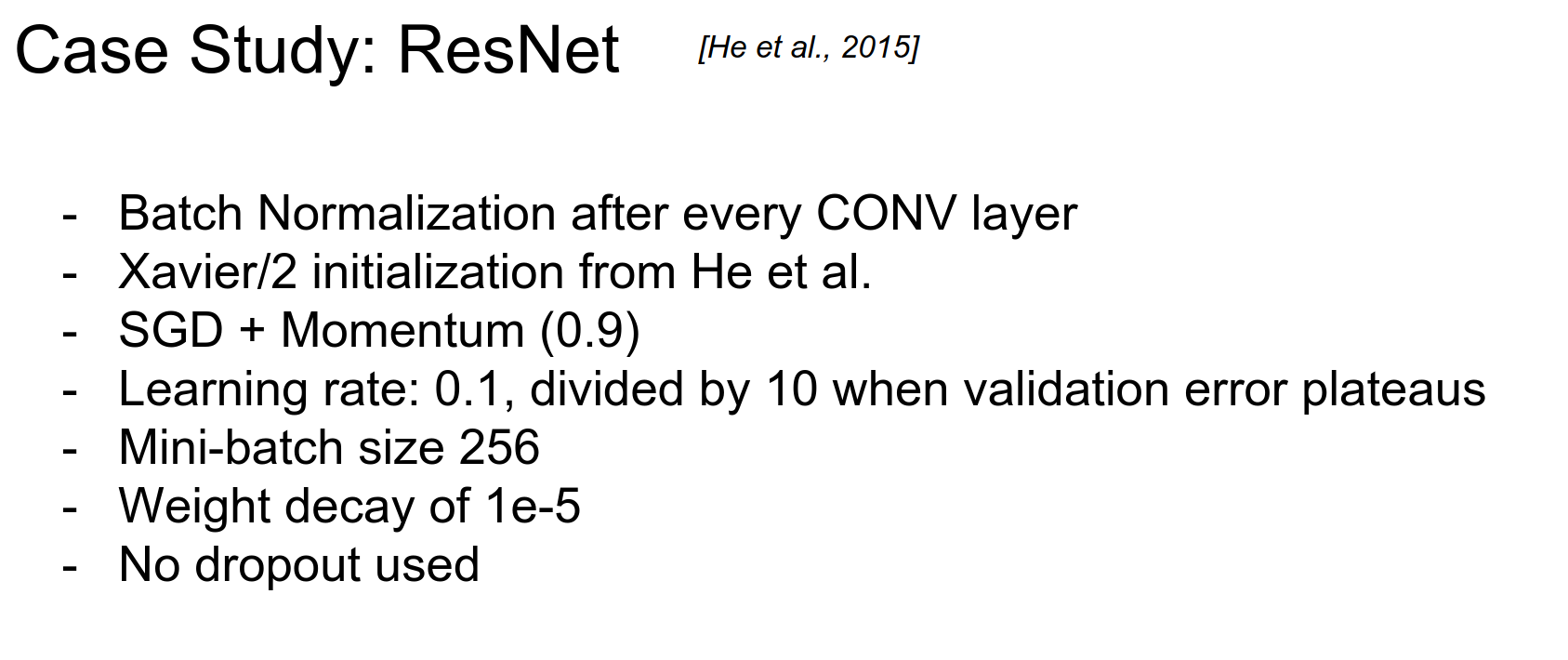
These are the commonly used hyperparameters.

• Batch norm layers will allow you to get away with a bigger learning rate.

• Using \(1x1\) Convs in clever ways.

This is the whole architecture; Andrej skipped it in the interest of time.

This was on the cover of AlphaGo.

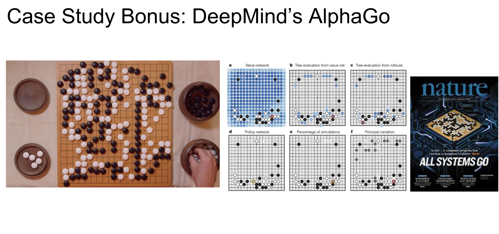
This was a convolutional network!

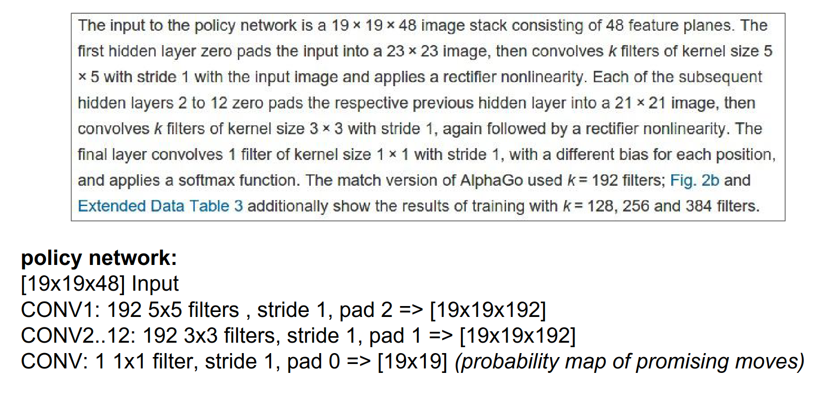
The input is \(19x19x48\) because they are using 48 different features based on the specific rules of Go. You can understand what is going on when you read the paper.

Other Go Deep Learning player: CrazyStone

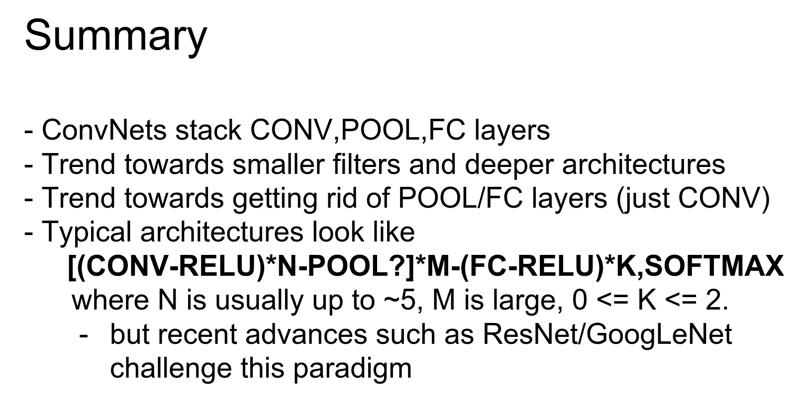
• The trend is to get rid of Pooling and Fully Connected Layers.

• Smaller filters and deeper architectures.

Done with lecture 7!