8. ConvNets for spatial localization, Object Detection

Part of CS231n Winter 2016

---

Lecture 8: Spatial Localization and Detection

We will give Andrej a little break.

Assignment 2 is due on Friday. The midterm is coming up.

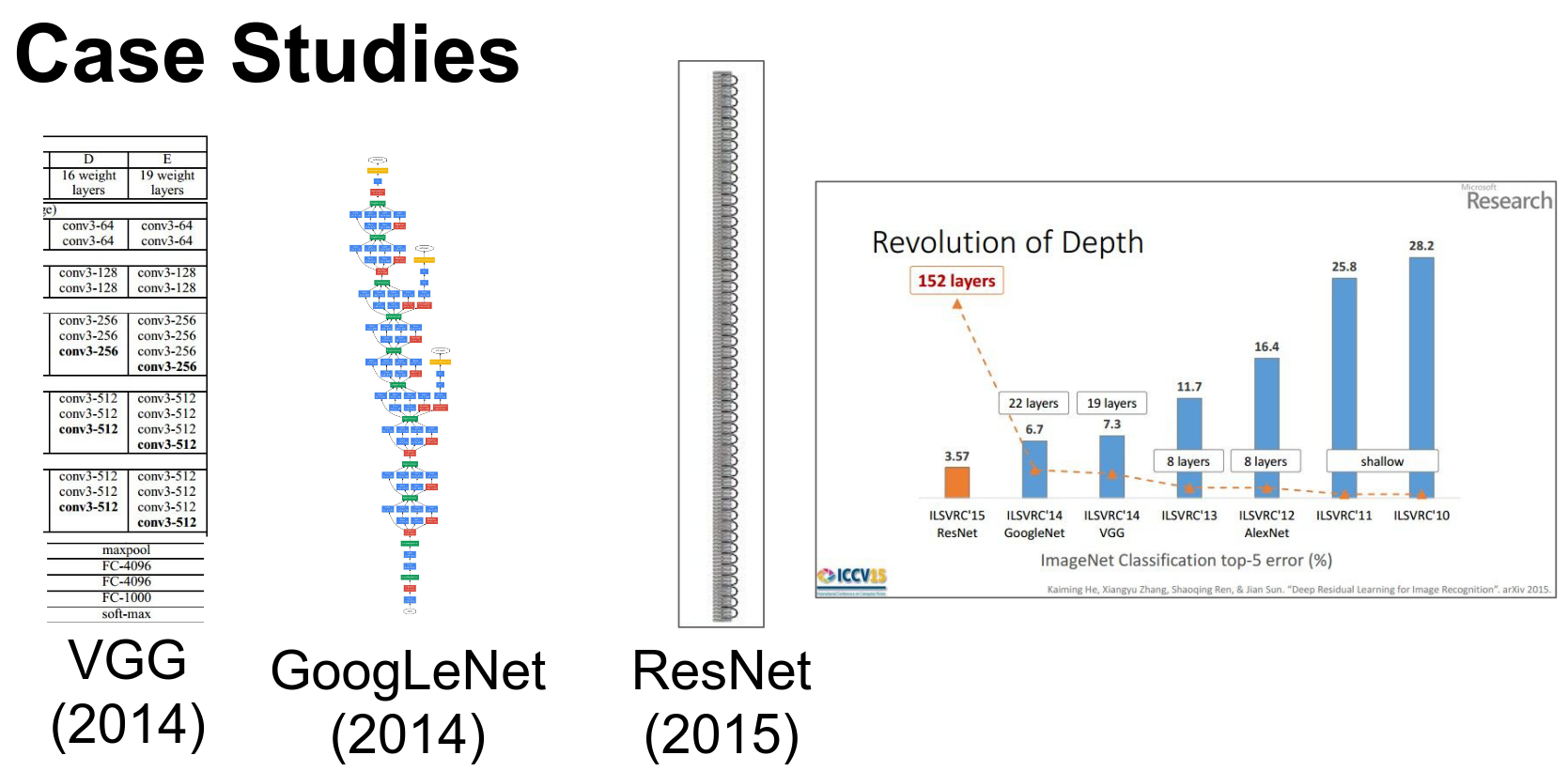
We talked about Convolutional Networks. Lower-level features appear early (low levels), and high-level features appear deeper (higher layers).

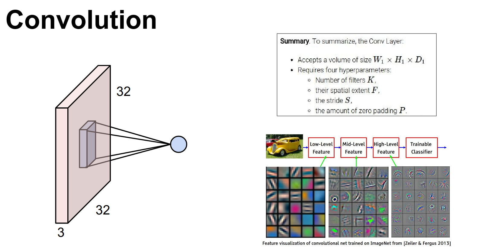
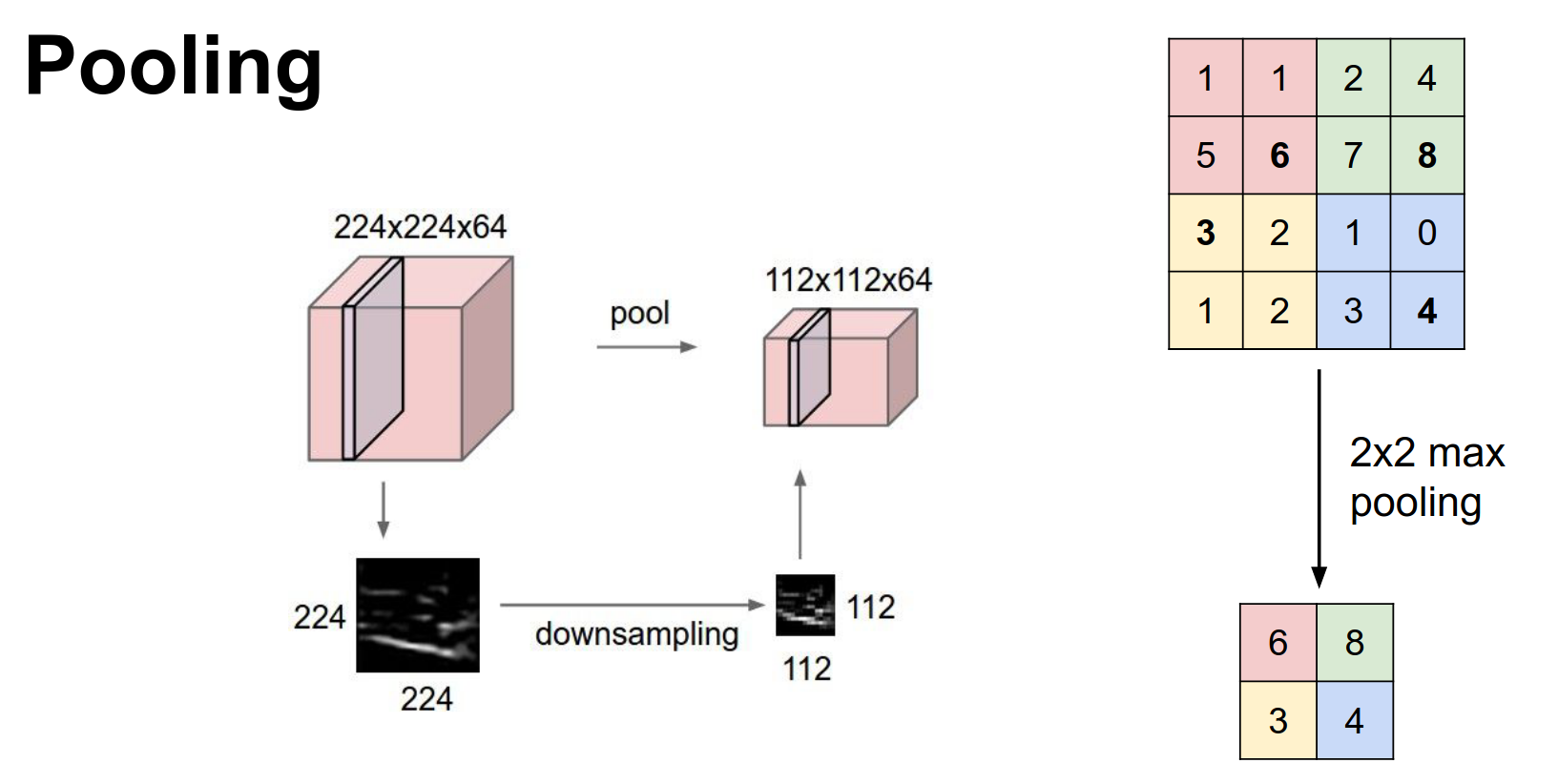
We saw pooling for shrinking spatial dimensions.

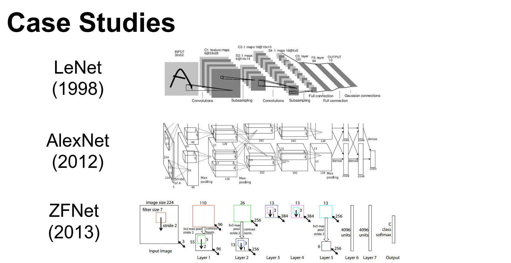
We saw a bunch of networks and how they are implemented.

We saw ResNet and how it changed the game.

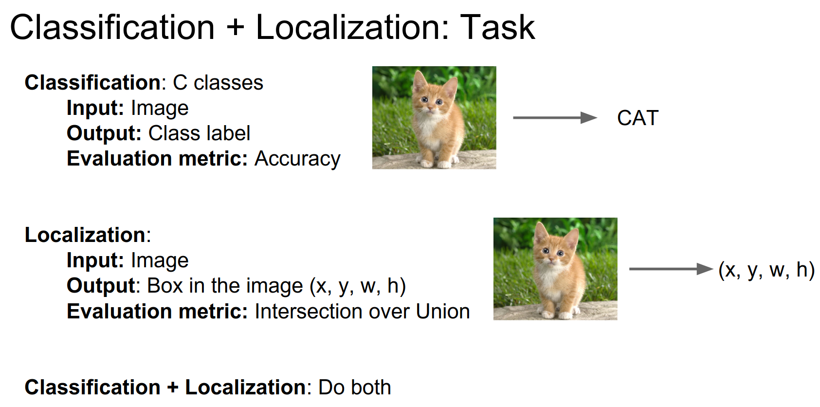
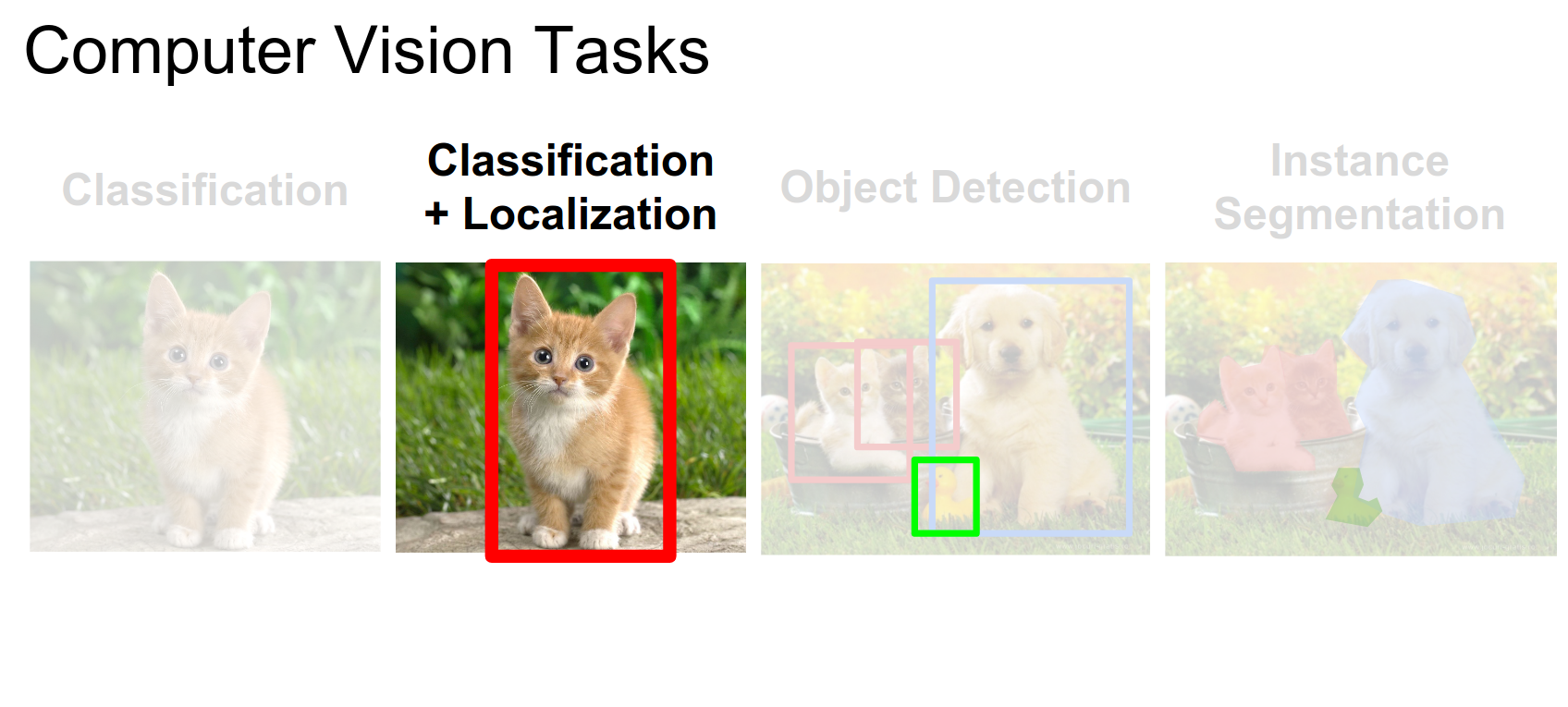
Localization and Detection

This is another big problem we have.

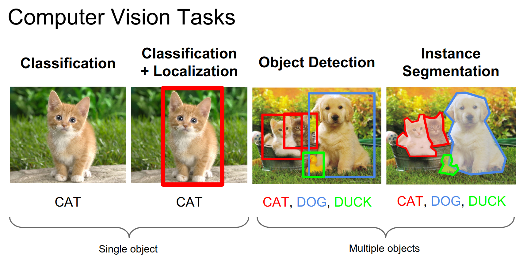
Localization asks: where exactly is the class? Detection is for bounding boxes, while instance segmentation finds contours around objects.

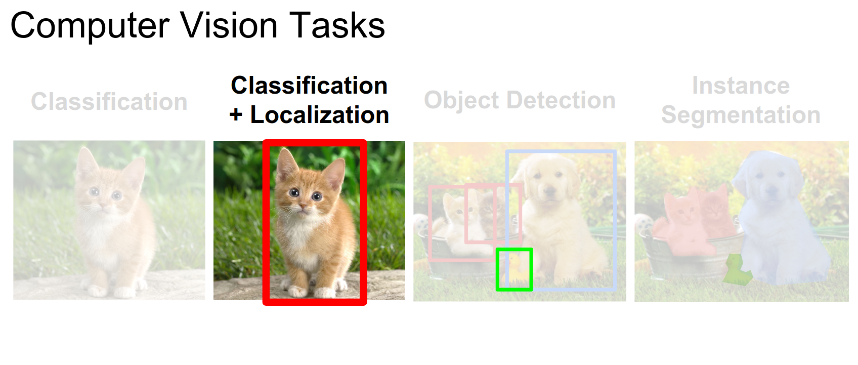
We can do both at the same time.

ImageNet also has this as a challenge.

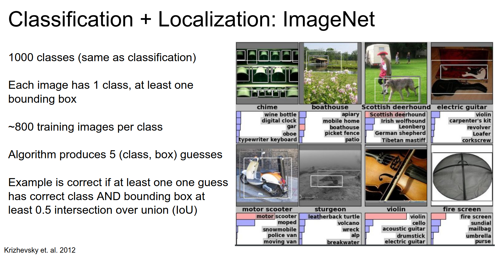
The class should be correct, and the Intersection over Union (IoU) should be over \(0.5\).

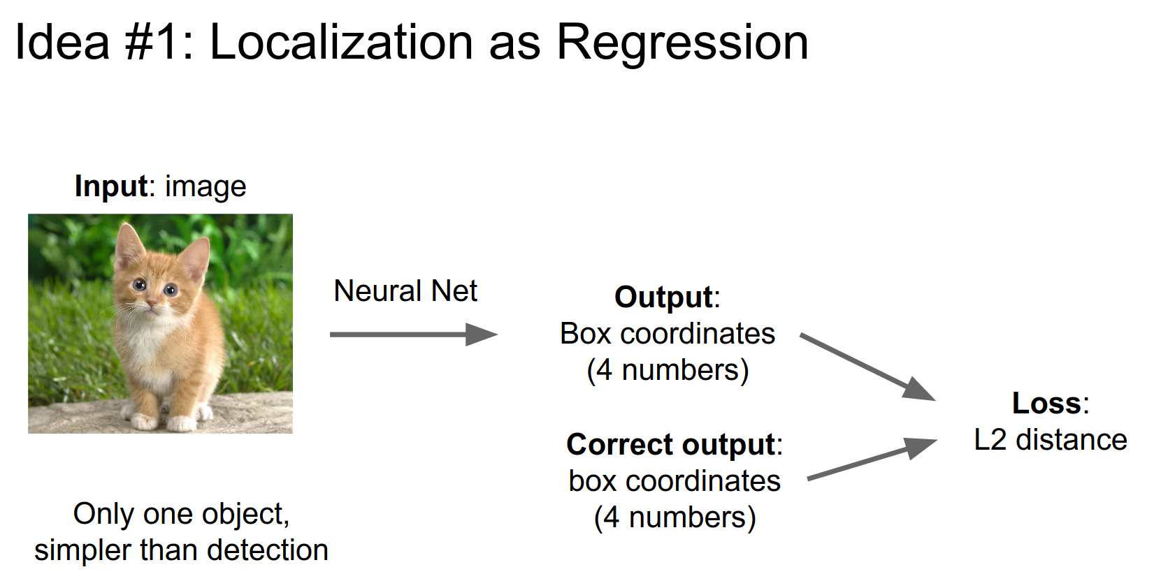
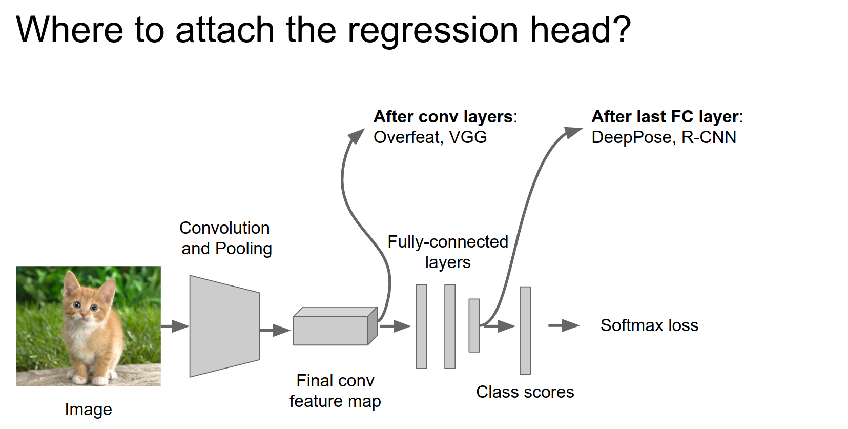
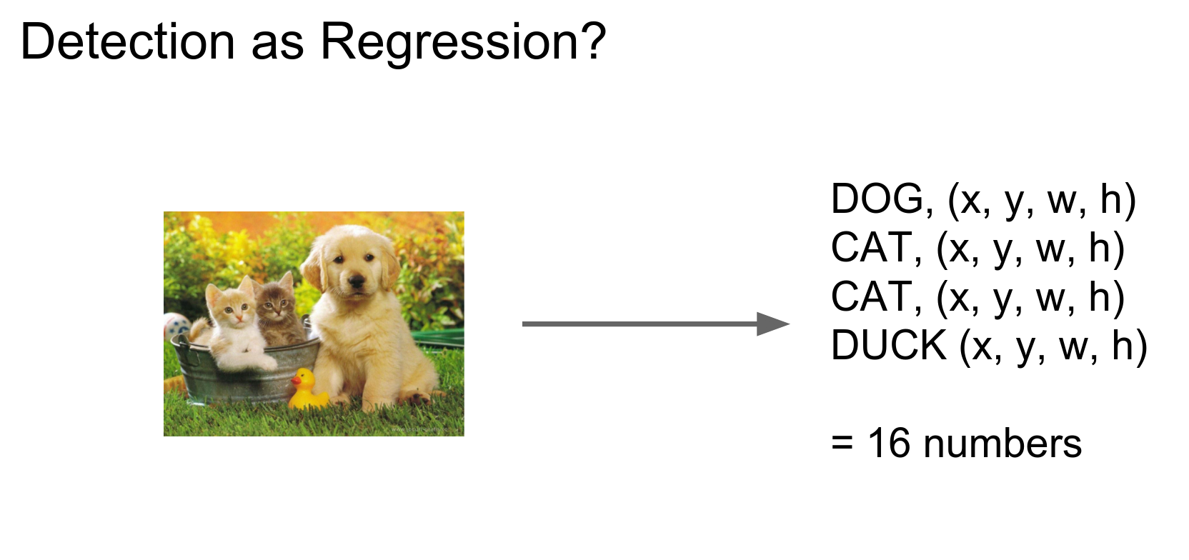
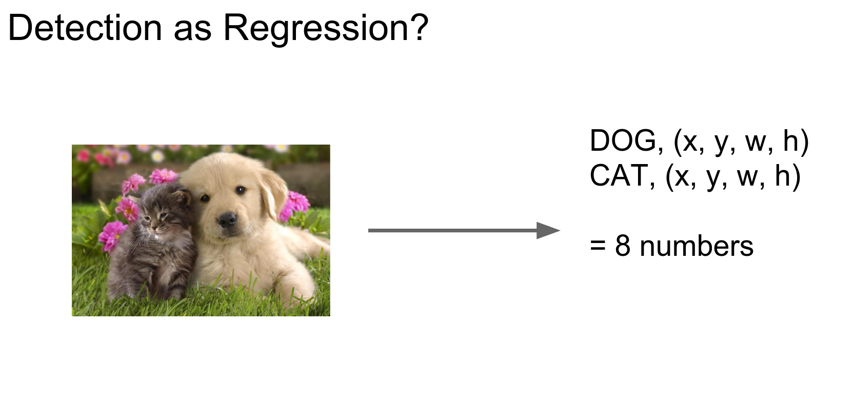
We can view localization as a regression problem where we generate 4 numbers.

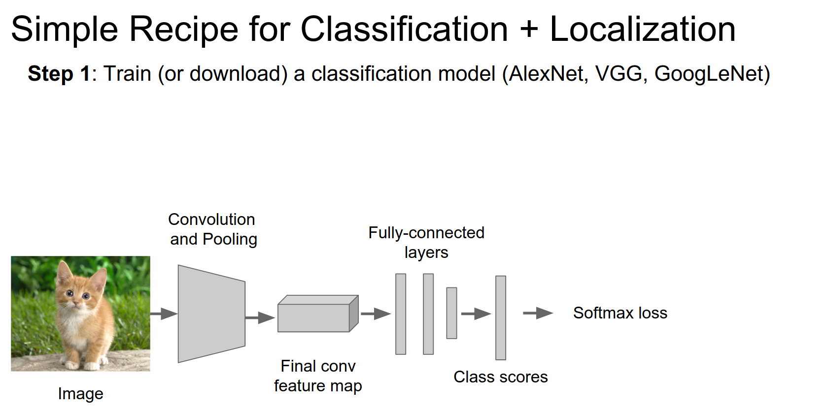
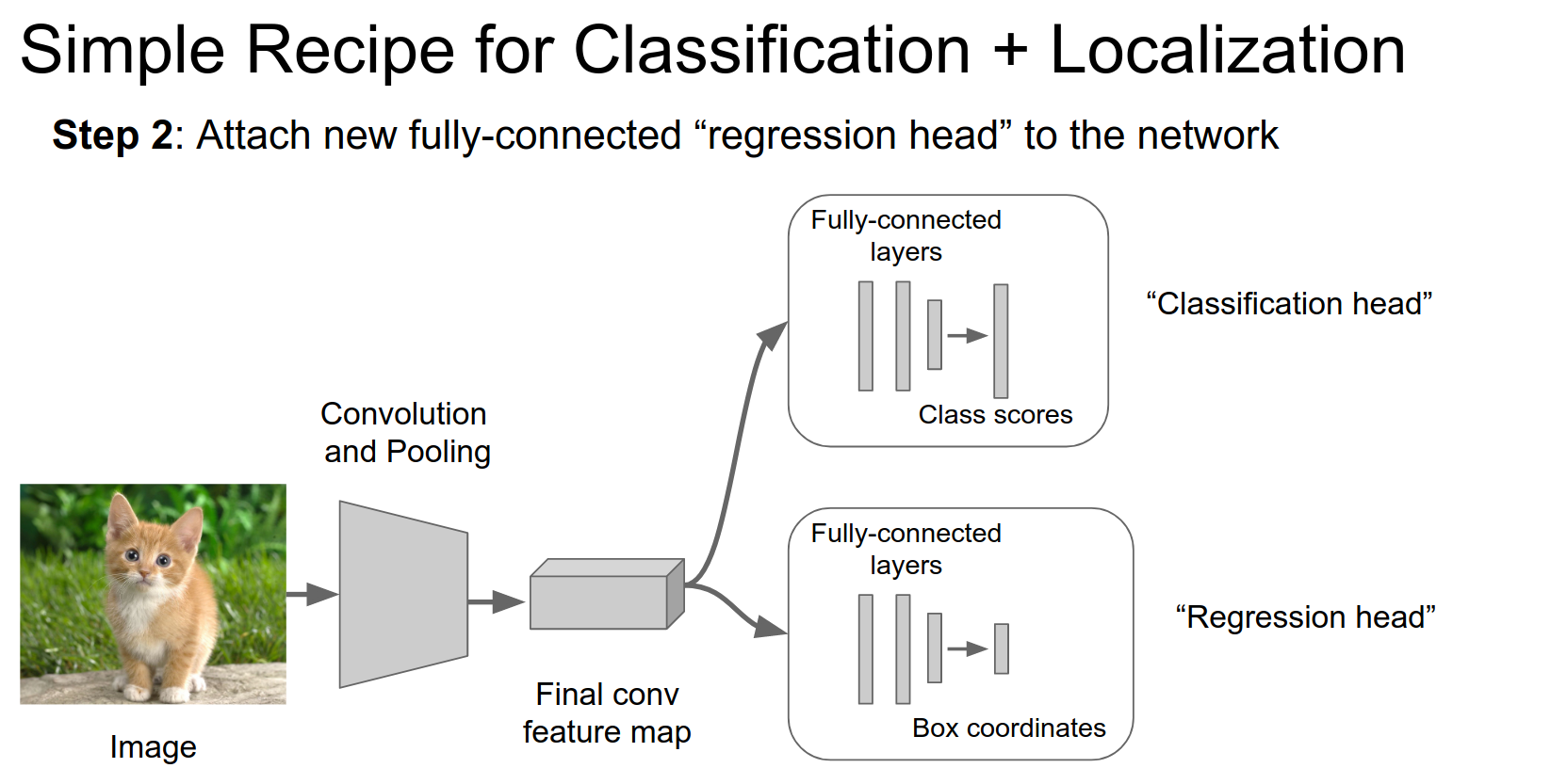
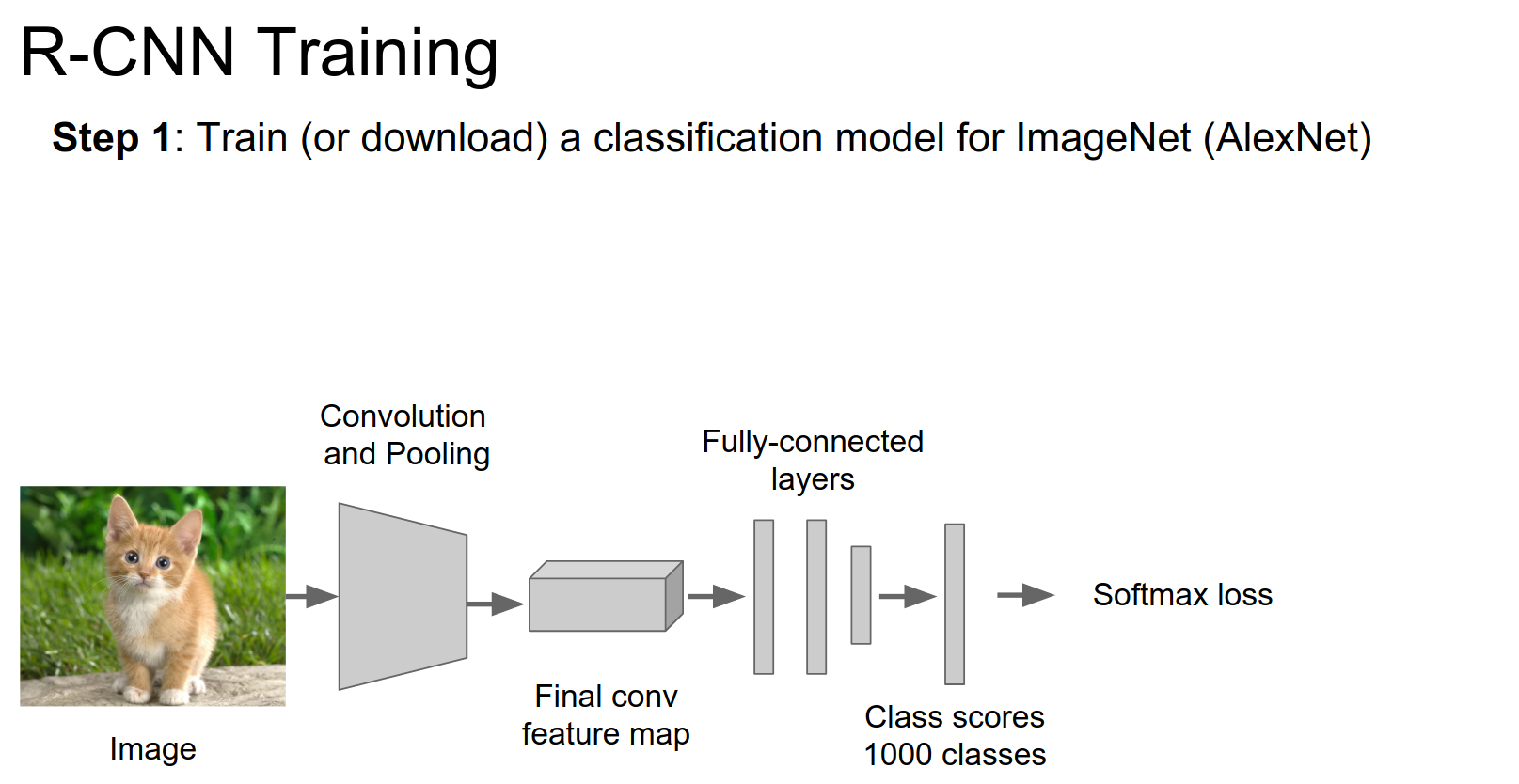
This is a simple recipe: take AlexNet or VGG, and download a pretrained model.

Take those fully connected layers that give us class scores and set them aside.

Attach new FC layers to some point in the network. This is the regression head. It's basically the same thing: a couple of FC layers outputting some real-valued numbers.

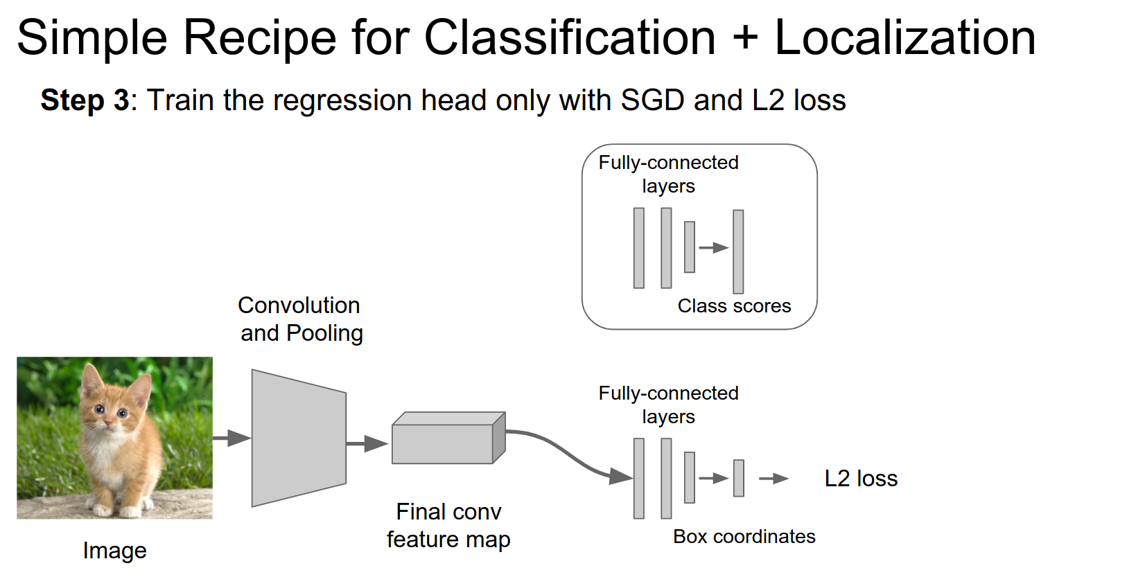
We train this just like we trained the classification network.

Loss Function

We train this network exactly the same way.

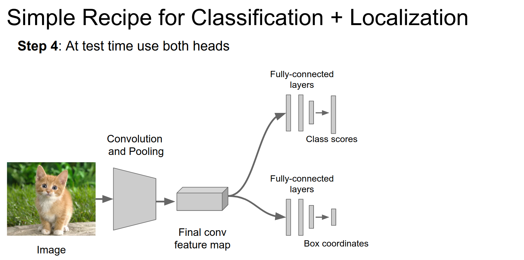
At test time, we use both heads to do classification and localization. We pass an image through the network (where we have trained both the classification and localization heads), get class scores and boxes, and we are done!

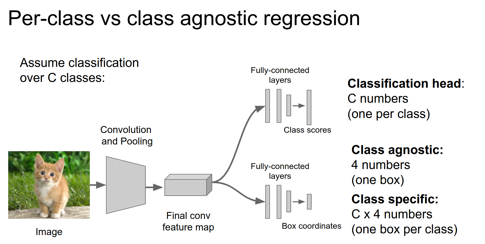
One detail: there are two main ways to do regression.

Just 4 numbers (class agnostic) or one bounding box per class.

Maybe attach it after the last convolutional layer, or after the last Fully Connected layer.

You could just attach it anywhere.

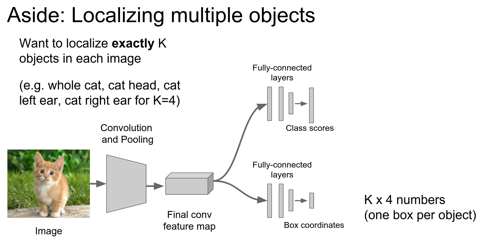
We are also interested in localizing multiple objects.

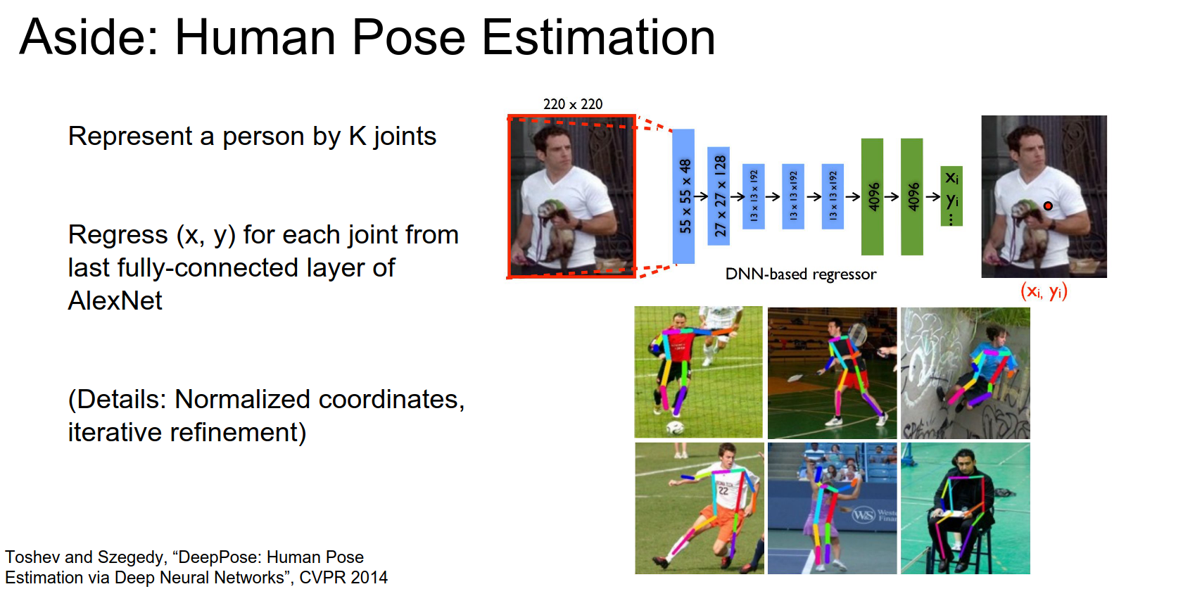
This is used in human pose estimation.

There is a fixed number of joints in a human. What is the pose of the person?

We can find all the joints, run the image through a CNN, and find all points for joints \((x,y)\), which gives us a way to find the current pose of the human.

Overall, this idea of localization as regression for a fixed number of objects is simple.

This will work. But if you want to win competitions, you need to add a little bit of fancy stuff.

You still have this dual-headed network, and you will combine predictions.

The classification head gives us class scores. The regression head gives us bounding boxes.

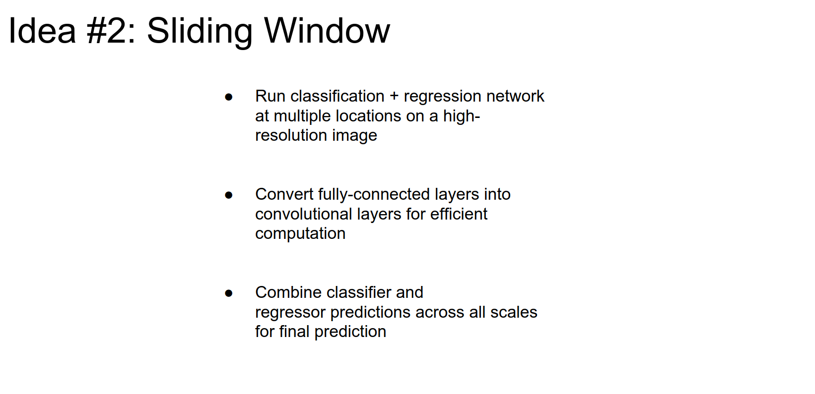
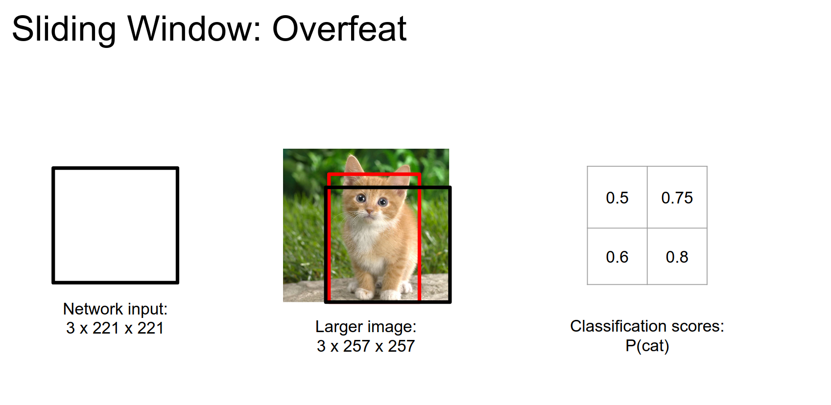
Sliding Window 🎈

If we run the window only on the upper right corner of the image, we will get a class score and a bounding box. We will repeat this on all 4 corners.

Corner top right:

Corner bottom left:

Corner bottom right:

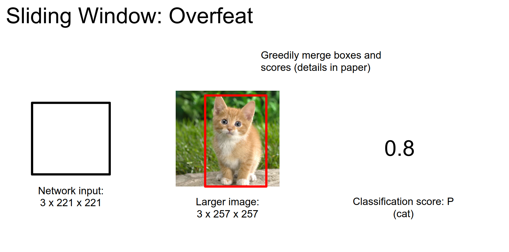
Bounding Box Merging

We only want a single bounding box. We greedily merge boxes (details in the paper).

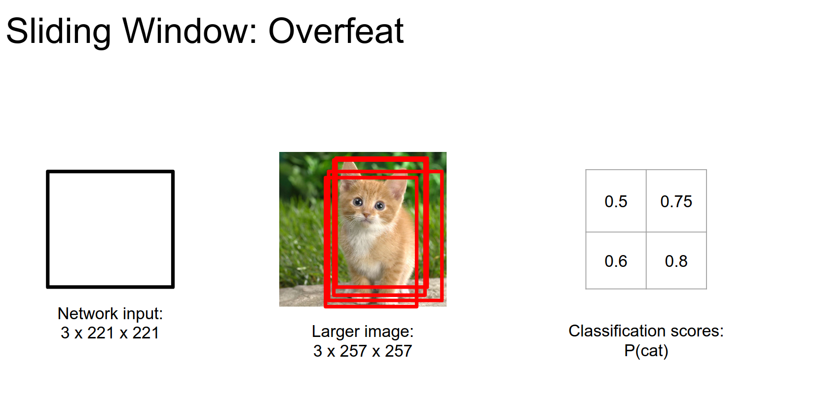
In practice, they used many more than 4 corners. The figure from the paper is below.

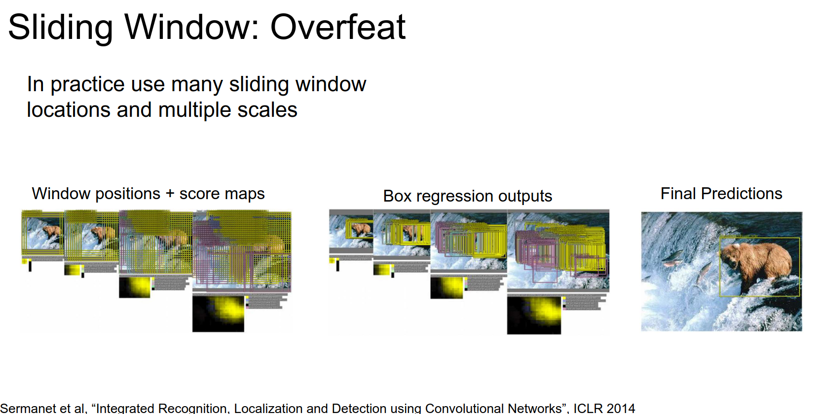
They finally decide on the best one.

It is pretty expensive to run the network on all crops.

Let's think about networks, convolutions, and Fully Connected layers.

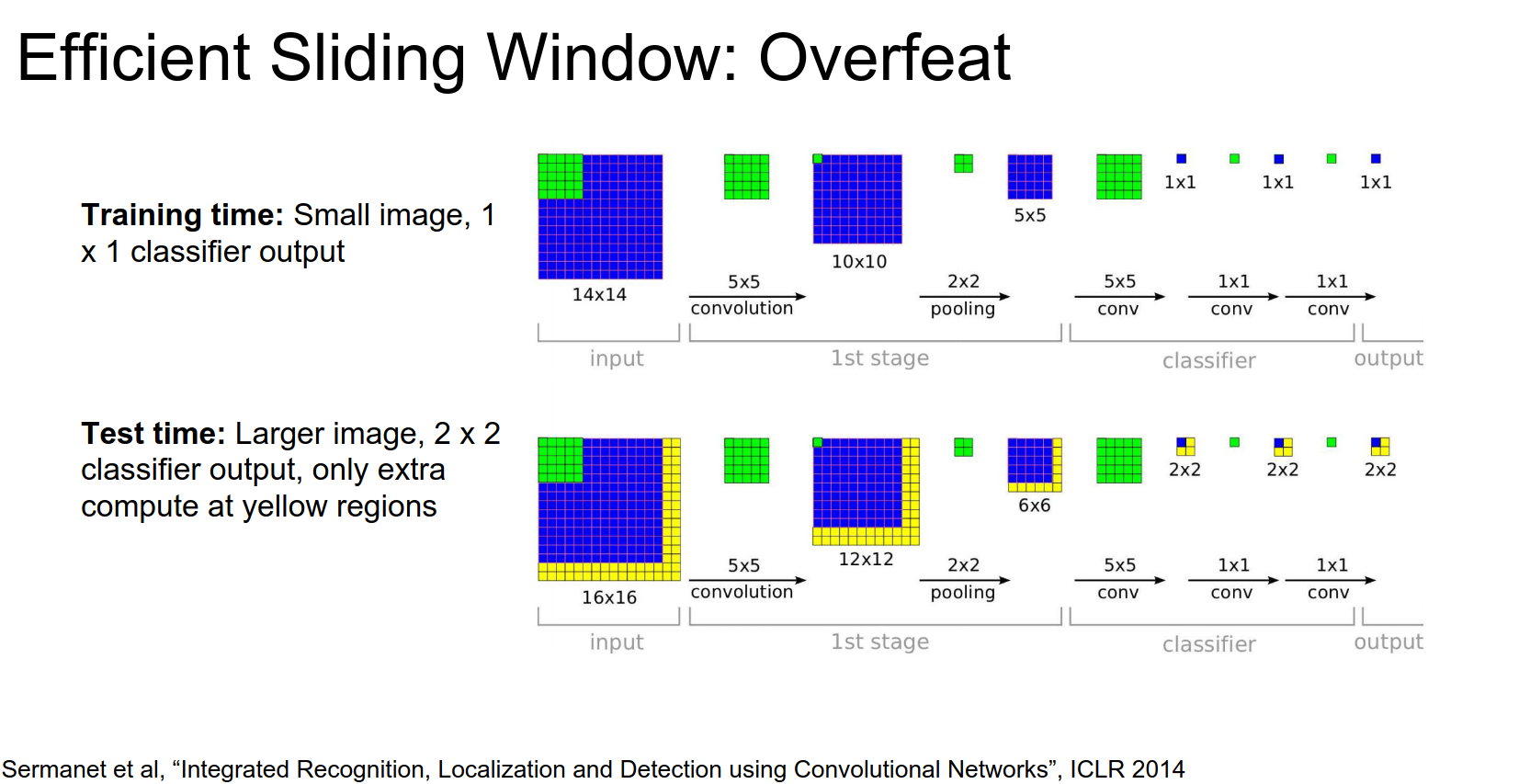
Fully Convolutional Networks

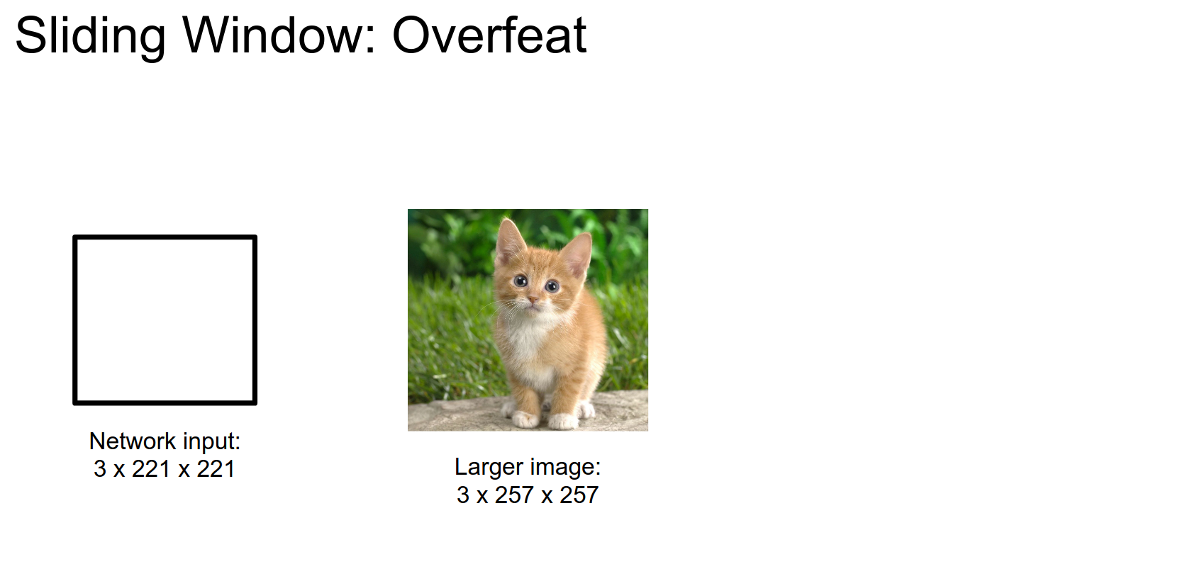
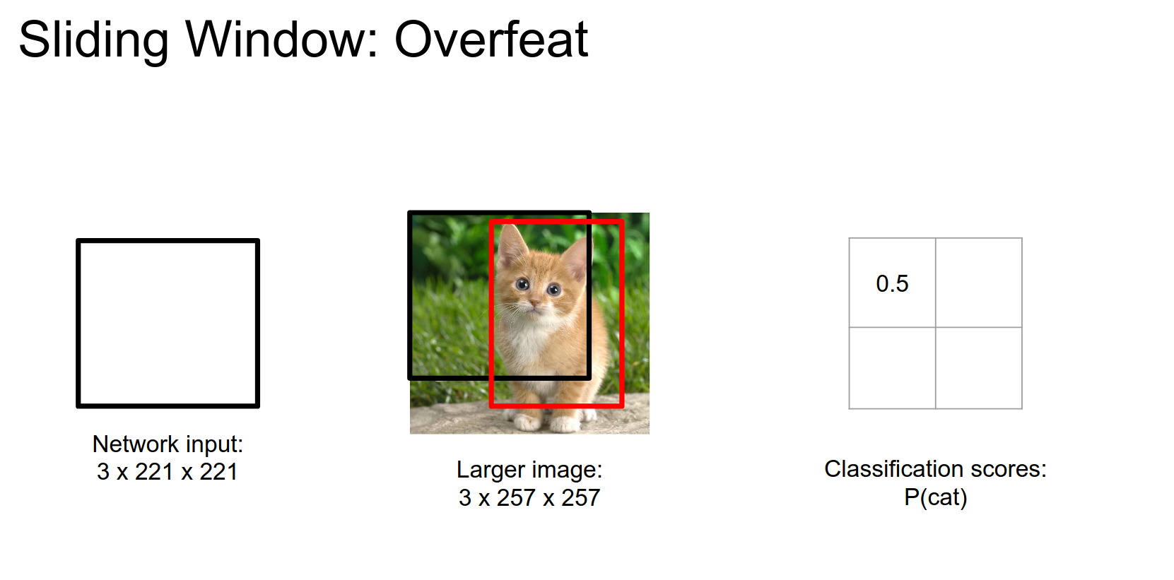
Now our network consists only of convolutions, pooling, and element-wise operations. We can now run the network on different-sized images.

This will give us a cheap approximation of running the network on different locations.

We previously had 4096 FC units, but we now have \(1x1\) convolutional layers.

Now, if we are working on \(14x14\) input at training time, with no FC, we have \(1x1x4096\) convs.

We can share computation in this way. The only extra computation is in the yellow parts.

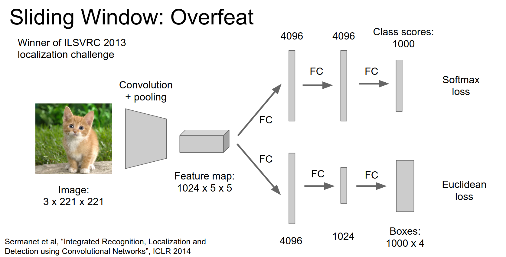
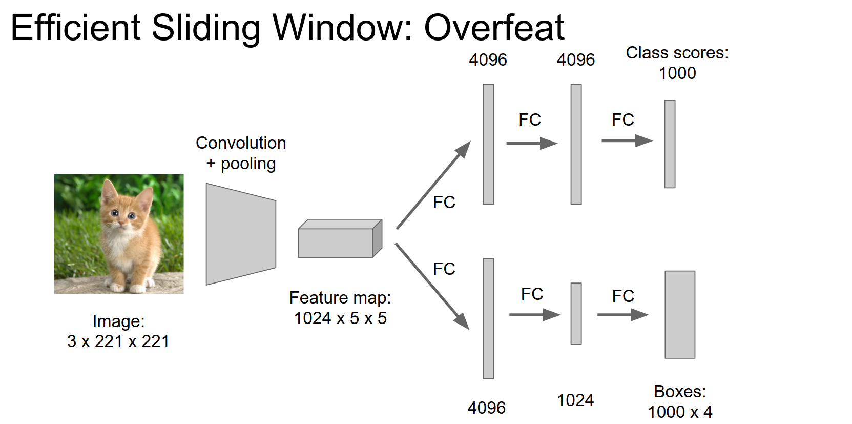
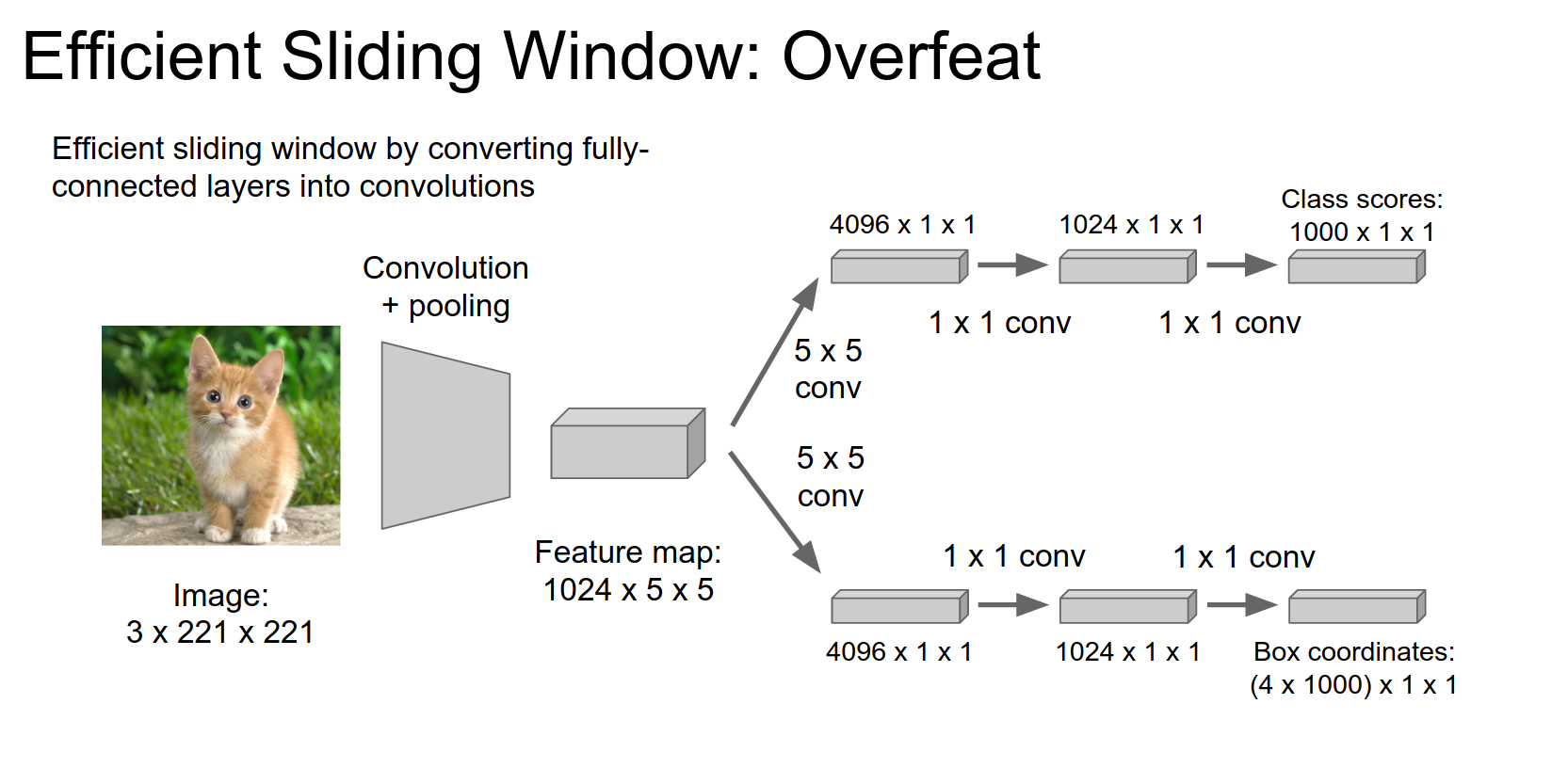
OverFeat 🪟

OverFeat uses a different architecture compared to traditional Convolutional Neural Networks (CNNs) by eliminating fully connected layers. Instead, it uses convolutional layers directly connected to the input image. This design choice allows OverFeat to process images of different sizes without the need for resizing or cropping.

By eliminating fully connected layers, OverFeat reduces the number of parameters in the model and avoids the computational overhead associated with processing high-dimensional feature vectors. This design simplifies the model and makes it more efficient, especially for tasks like object detection where processing speed is critical.

The point here isn't really 're-imagining' the FC layer as a convolution step. Instead, it lets you take advantage of efficiencies built into Convolution Operation implementations that aren't present in FC implementations.

Imagine a convolution operation in 1 dimension. Let's say your kernel is 5 numbers. In step 0, I add A+B+C+D+E = A + (B + C + D + E). That costs me 4 add ops. In step 1, I want to add B+C+D+E+F. I can use my cached value and calculate it with (cached_value) + F, which only costs me 1 add op. Efficiencies like this can be scaled to implementations of the convolution operator. However, FC layers operate over the whole input and have no logical place for such caching.

In OverFeat, we're running these operations on 'windows' of the input image. Each window is a lot like a patch of input to a convolutional layer. By transforming the last FC layers into convolution operations, we can treat the whole network as a series of convolution operations and then take advantage of the inherent efficiencies (described above) of convolution operations.

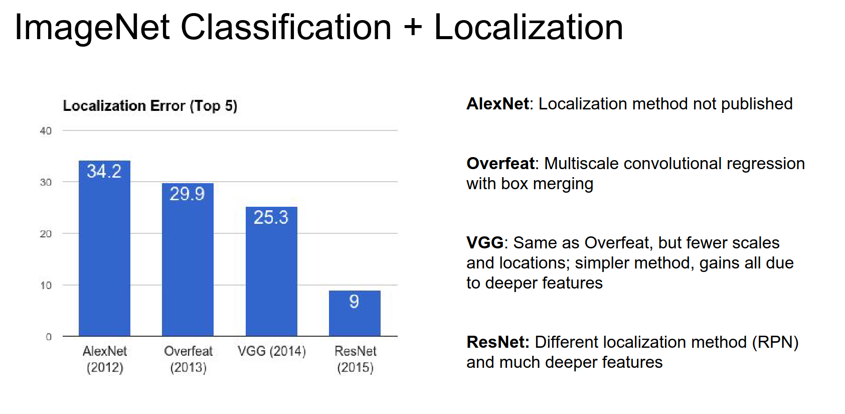
In the classification + localization problem, the 2013 winner used the OverFeat method.

VGG used a deeper network, and it improved the results.

ResNet crushed the competition. They used a different localization method: RPNs.

Now we move on.

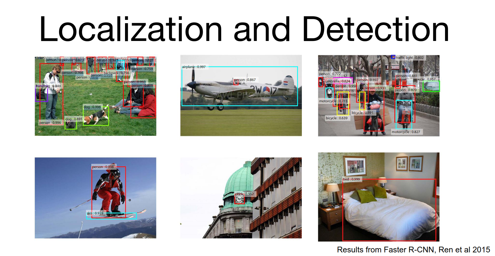
Object Detection 🐱 🐶

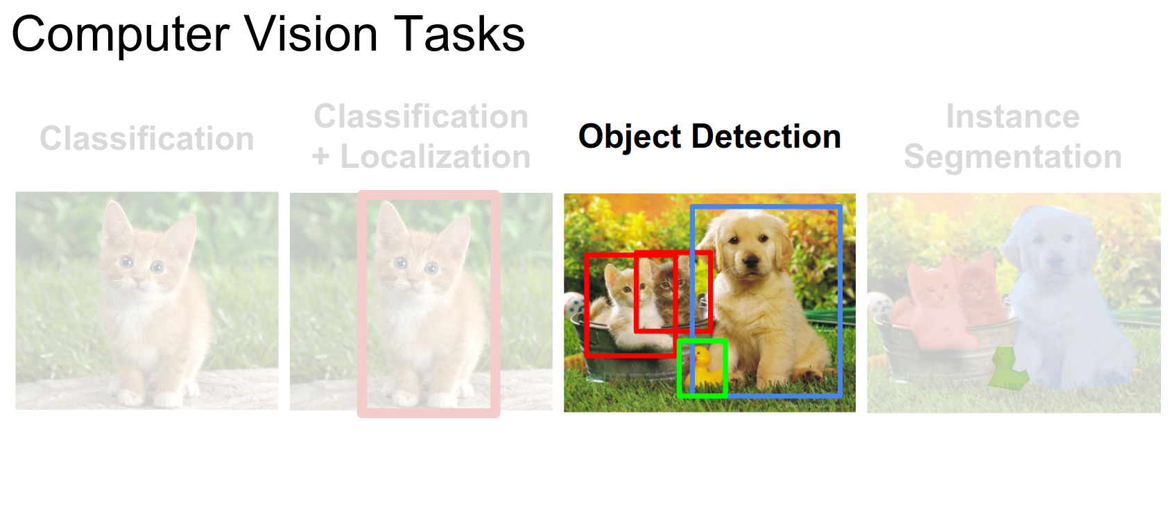
Can we use regression here too?

2 classes.

n cats - \(nx4\) coordinates.

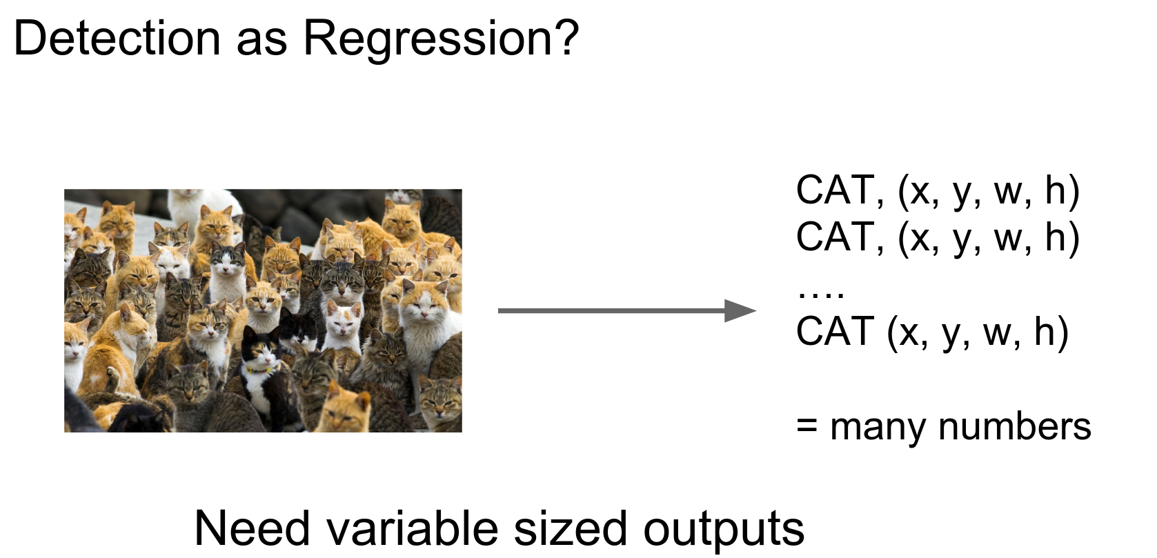
We need something different because we have variable-sized outputs.

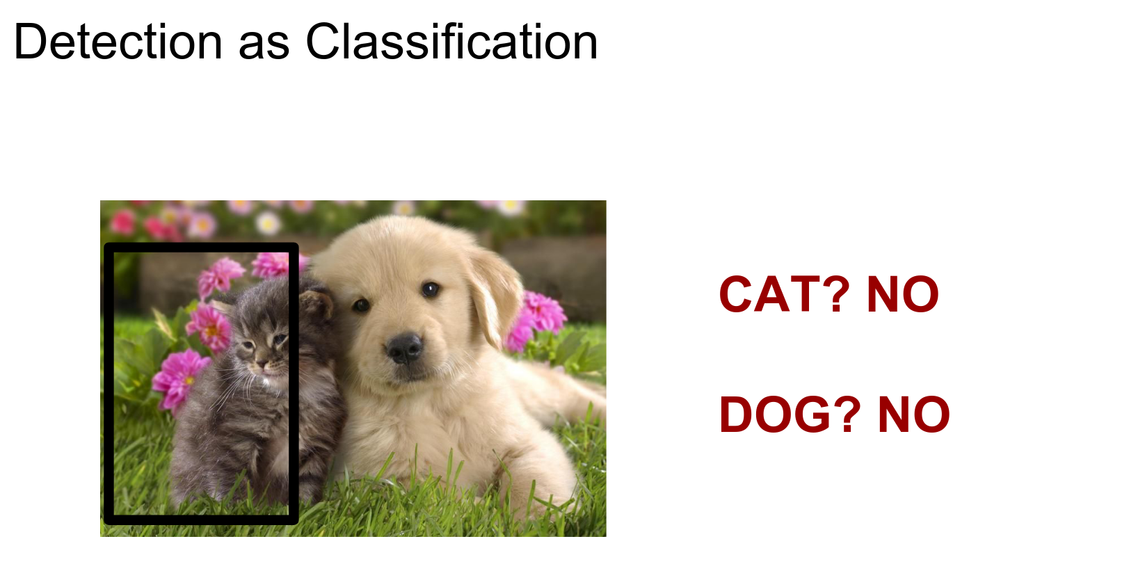
You have 2 blades: regression and classification. If regression did not work, try classification.

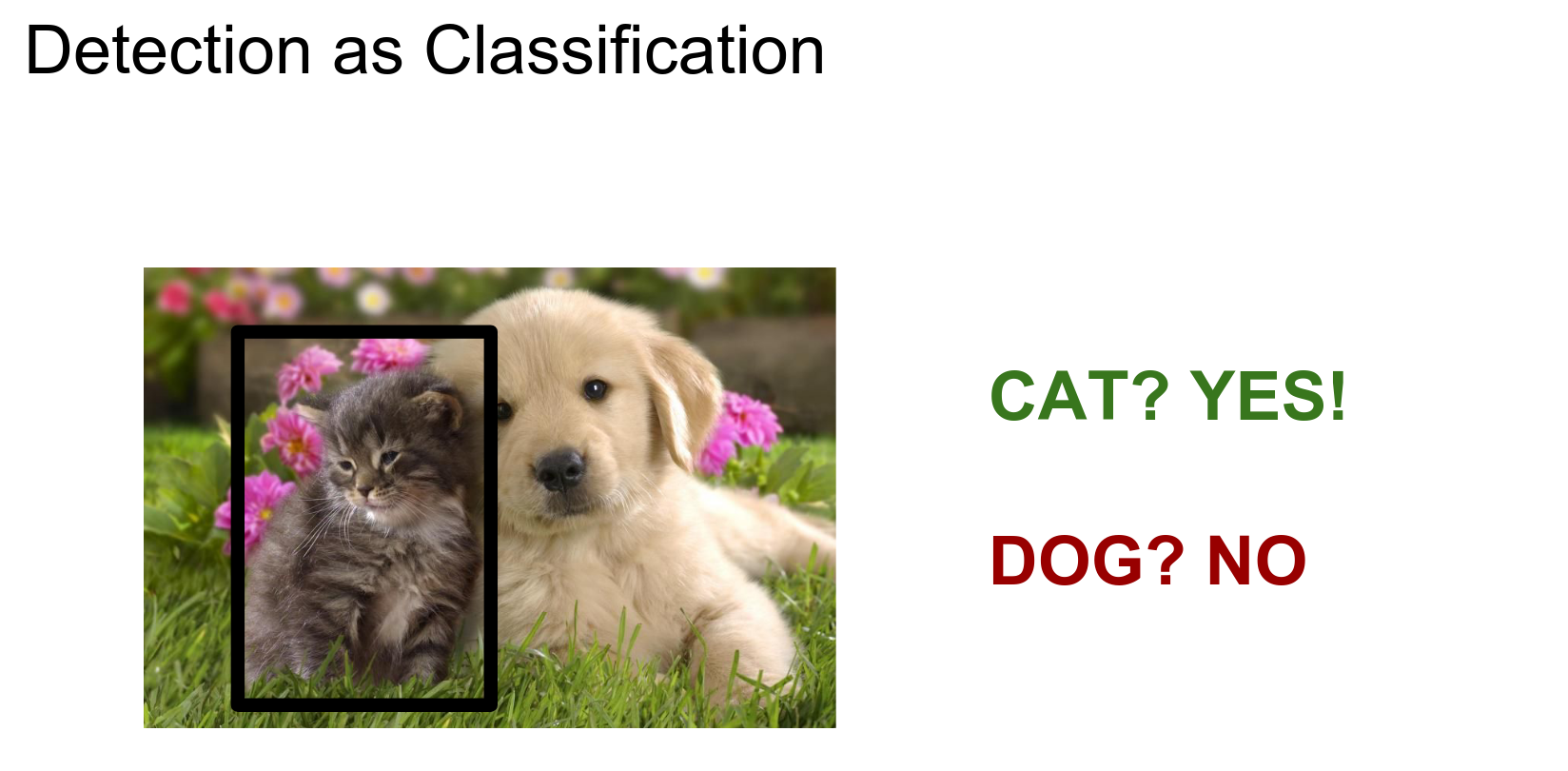
Found a cat here!

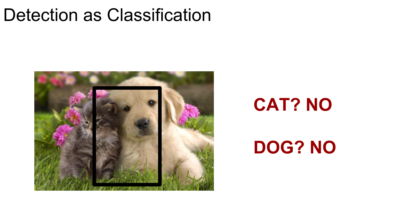
Nothing here.

So what we do is try out different image regions, run a classifier on each one, and this will solve the variable-sized output problem.

Exhaustive Search

Detection is a really old problem in Computer Vision, which was solved by HoG in 2005 for pedestrians.

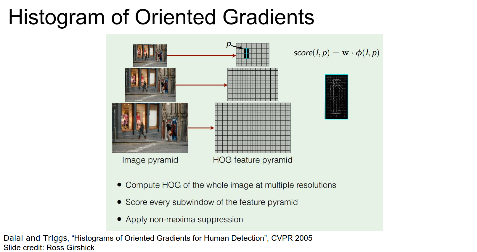
Do linear classifiers; they are fast. Run a Linear Classifier at every scale at every position.

• Compute HoG of the entire image at multiple resolutions.
• Score every sub-window of the feature pyramid.
• Apply non-maxima suppression.

People took this idea and worked on it. One of the most important paradigms before deep learning was:

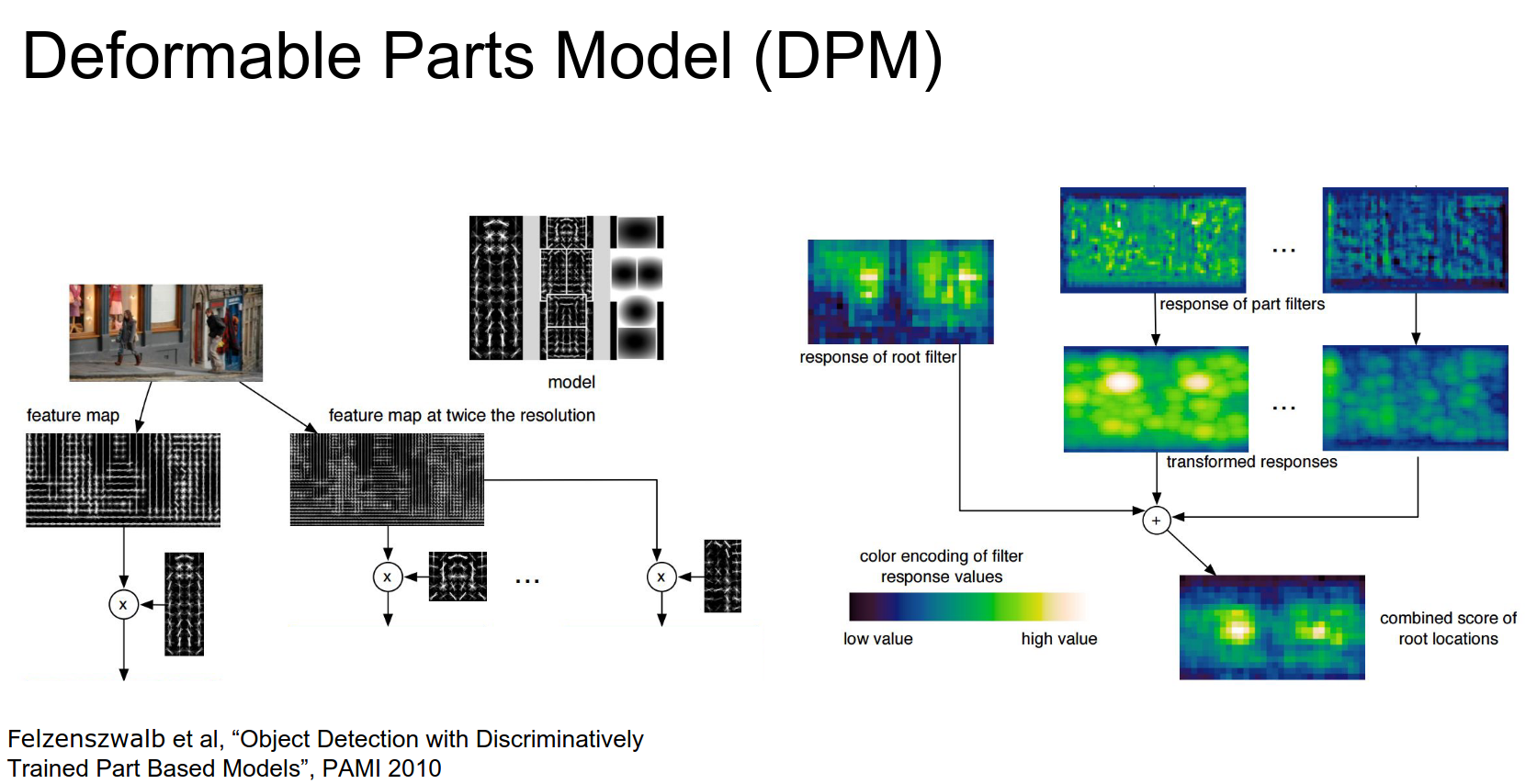
Deformable Parts Model

We are still working on HoG features, but instead of a simple linear classifier, we have a linear template for objects that varies over spatial positions.

Latent SVM is used here.

It is a more powerful classifier. It still works really fast. We still run it everywhere at every scale.

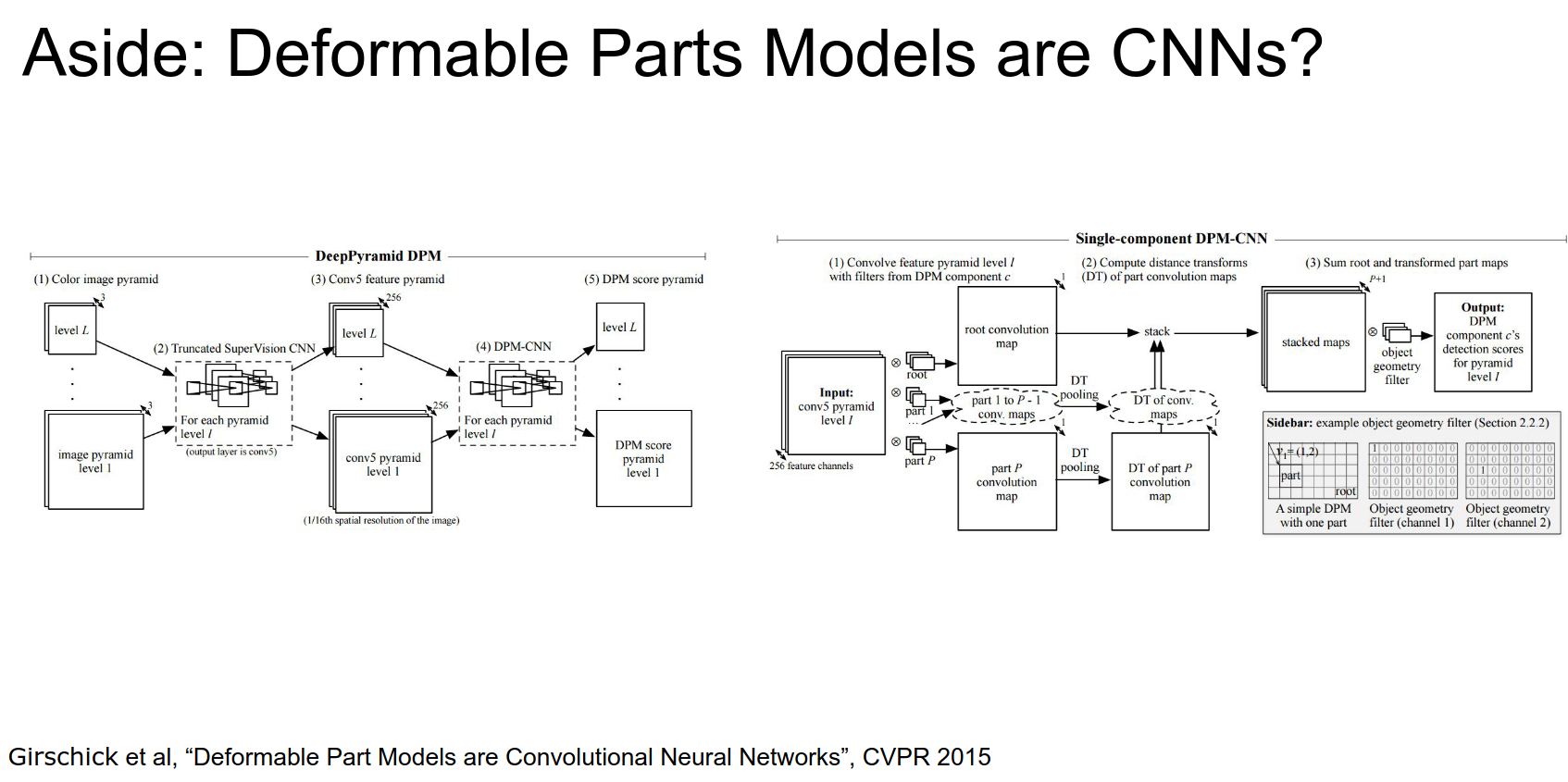
These are just ConvNets.

HOG vs CNN - Histogram is kinda like pooling, edges are like convolutions.

We still have a problem.

We use an expensive classifier on certain regions!

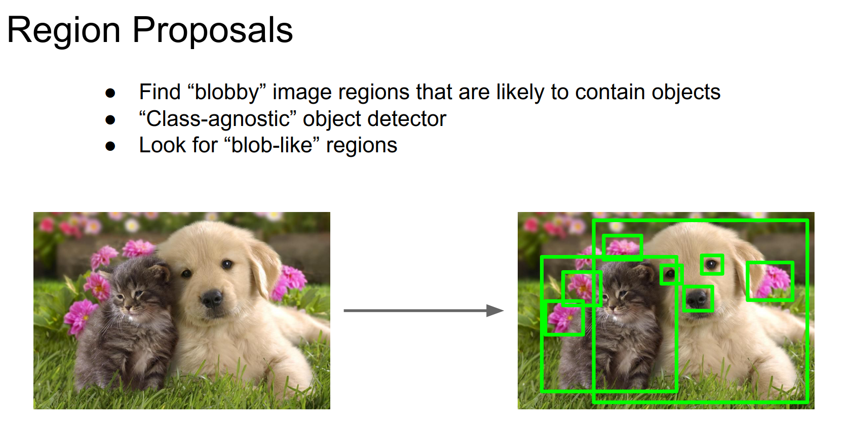
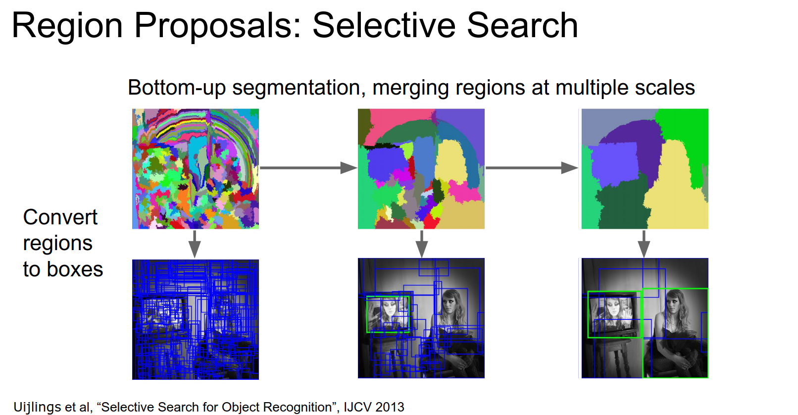
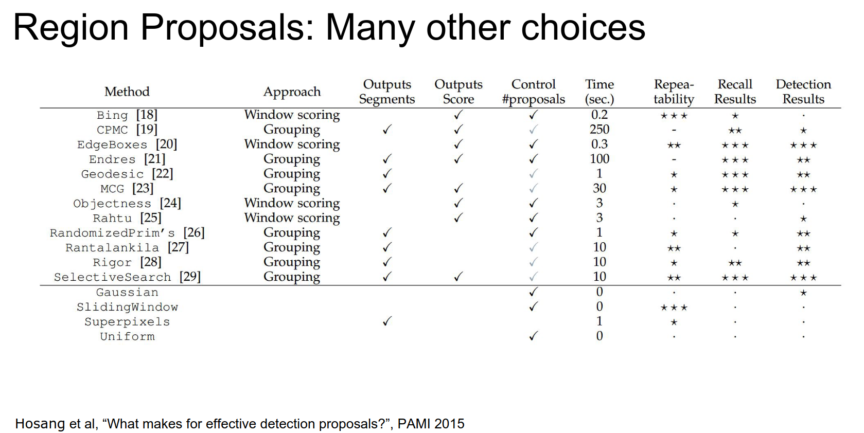
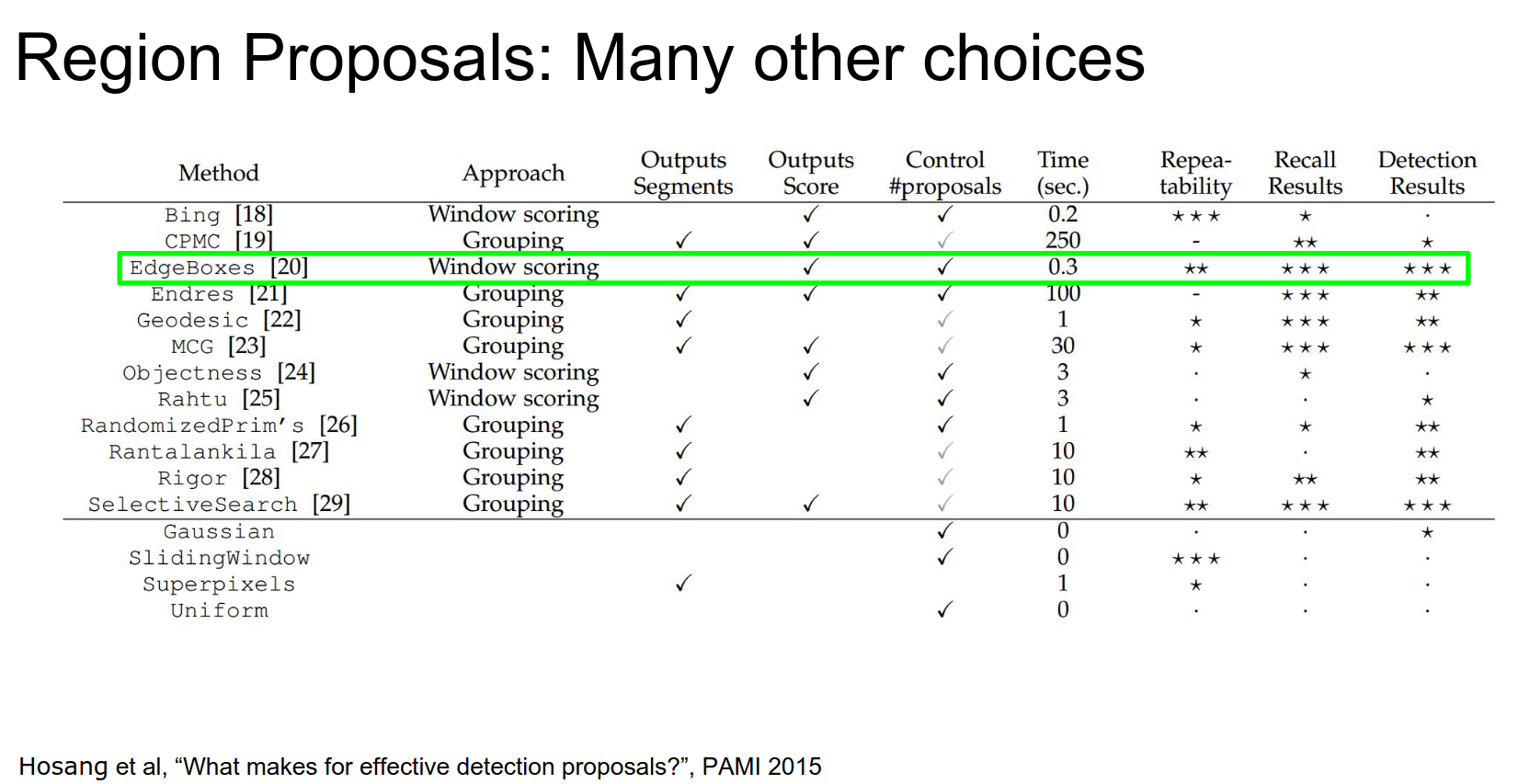
Region Proposals 🤹

They do not care about classes; they are looking for blob-like structures. They just run FAST.

The most famous one is called Selective Search:

Here is more information about selective search. Here is a Python Package for it.

You start from pixels, merge adjacent pixels if they have similar color and texture, and form connected blob-like features.

After that, you can convert these regions into boxes.

There are a lot of different proposal methods. Tip: EdgeBoxes

---

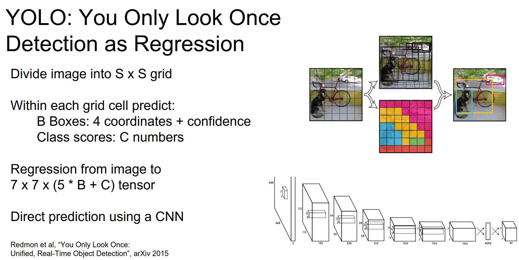
YOLO Overview

YOLO (You Only Look Once) does not utilize region proposals like some other object detection algorithms such as Faster R-CNN or R-CNN. Instead, YOLO performs object detection by dividing the input image into a grid of cells and predicting bounding boxes and class probabilities directly from each grid cell.

Here's a brief overview of how YOLO works:

• Grid Division: YOLO divides the input image into a grid of cells. Each cell is responsible for predicting bounding boxes and class probabilities for the objects contained within it.
• Bounding Box Prediction: For each grid cell, YOLO predicts bounding boxes. Each bounding box is represented by a set of parameters: (x, y) coordinates of the box's center relative to the grid cell, width, height, and confidence score. The confidence score indicates how likely the bounding box contains an object and how accurate the box is.
• Class Prediction: Along with each bounding box, YOLO predicts class probabilities for the objects present in the bounding box. This is done using softmax activation to estimate the probability of each class for each bounding box.
• Non-Maximum Suppression (NMS): After obtaining bounding boxes and their associated class probabilities, YOLO applies non-maximum suppression to remove redundant or overlapping bounding boxes. This ensures that each object is detected only once with the most confident bounding box.

By directly predicting bounding boxes and class probabilities from grid cells without the need for region proposals, YOLO achieves real-time object detection capabilities. This approach allows YOLO to detect objects efficiently in a single forward pass of the neural network.

---

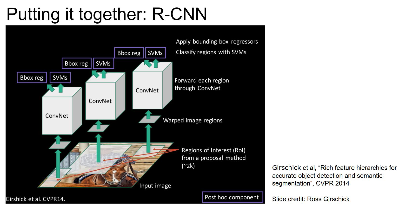
Let's put all of them together.

• We have an input image.
• We will run a region proposal method to get 2000 boxes.
• Crop and warp that image region to some fixed size.
• Run it through a CNN.
• The CNN will have a regression head.

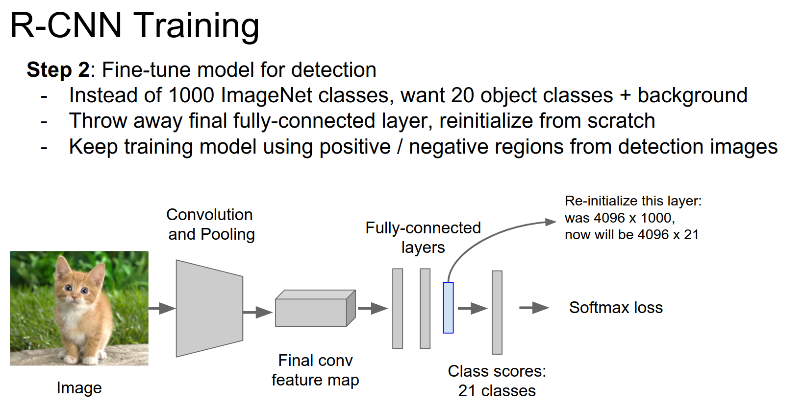
Training is a bit complicated. Download a pretrained classification model.

We need to add a couple of layers at the end.

We use positive and negative regions from detection images. Initialize a new layer and train again.

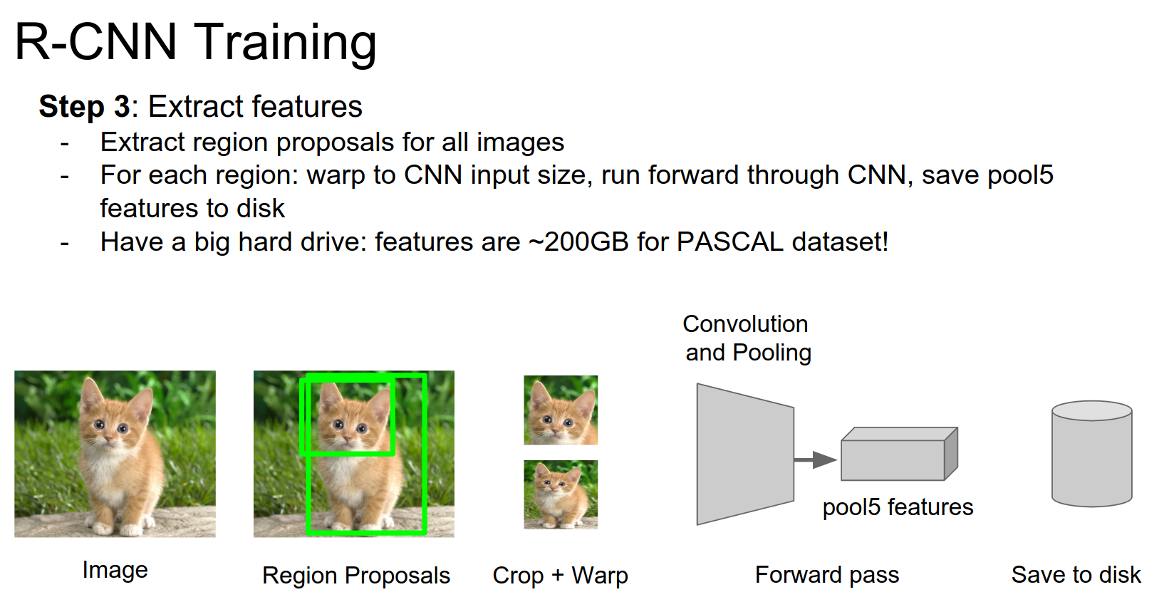
We want to cache all these features to disk. For every image in your dataset, you run selective search, extract the regions, warp them, and run them through a CNN.

And, you cache the features to disk.

Storage Requirements

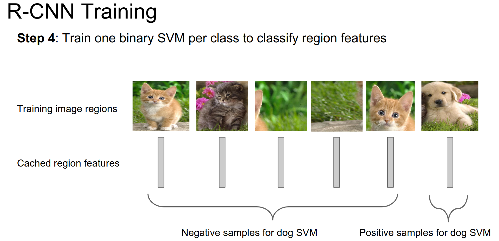
We want to train SVMs to be able to classify different classes based on the features.

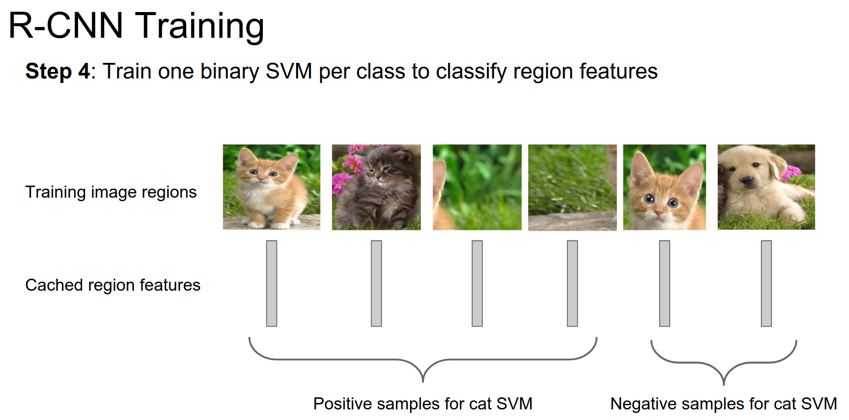
• You have these image regions.
• You have features for those regions.
• You divide them into positive and negative samples for each class.
• You train binary SVMs.

You do this for every class in your dataset.

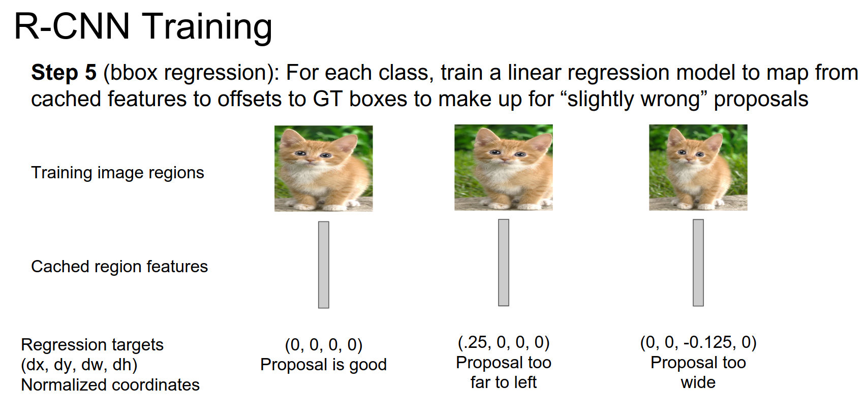
Bounding Box Regression

Your region proposals are not perfect. You might want to make corrections.

If the proposal is too far to the left, you need to regress to this correction vector.

They just do linear regression; you have features and targets, so you just train linear regression.

3 datasets are used in practice.

ImageNet has a lot of different images. One object per image.

COCO - a lot more objects per image.

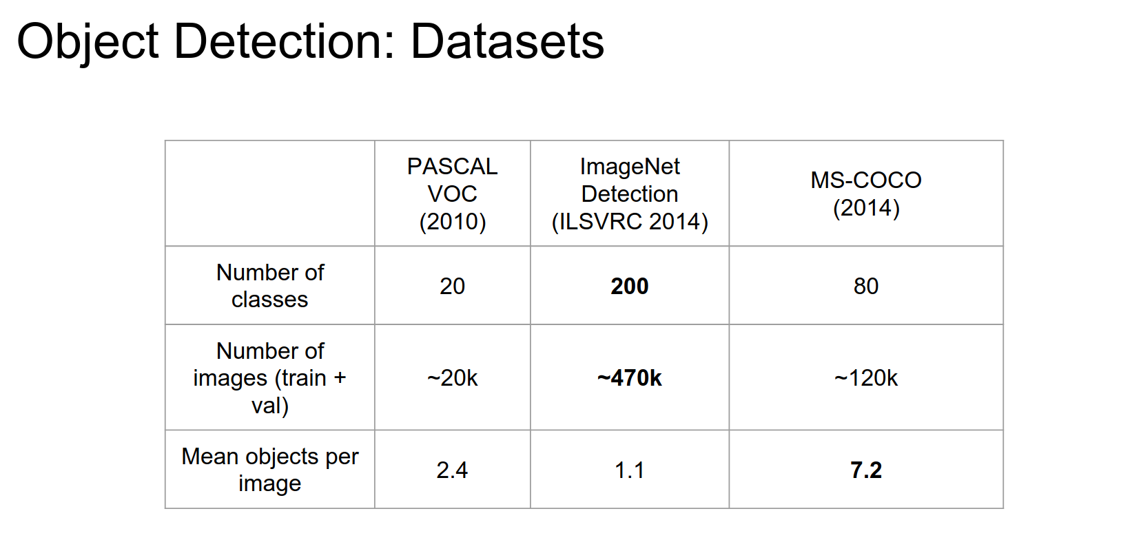
mAP is the main metric for detection.

PASCAL dataset, 2 different versions. Publicly available, so easier to use.

Feature Extraction 🍒

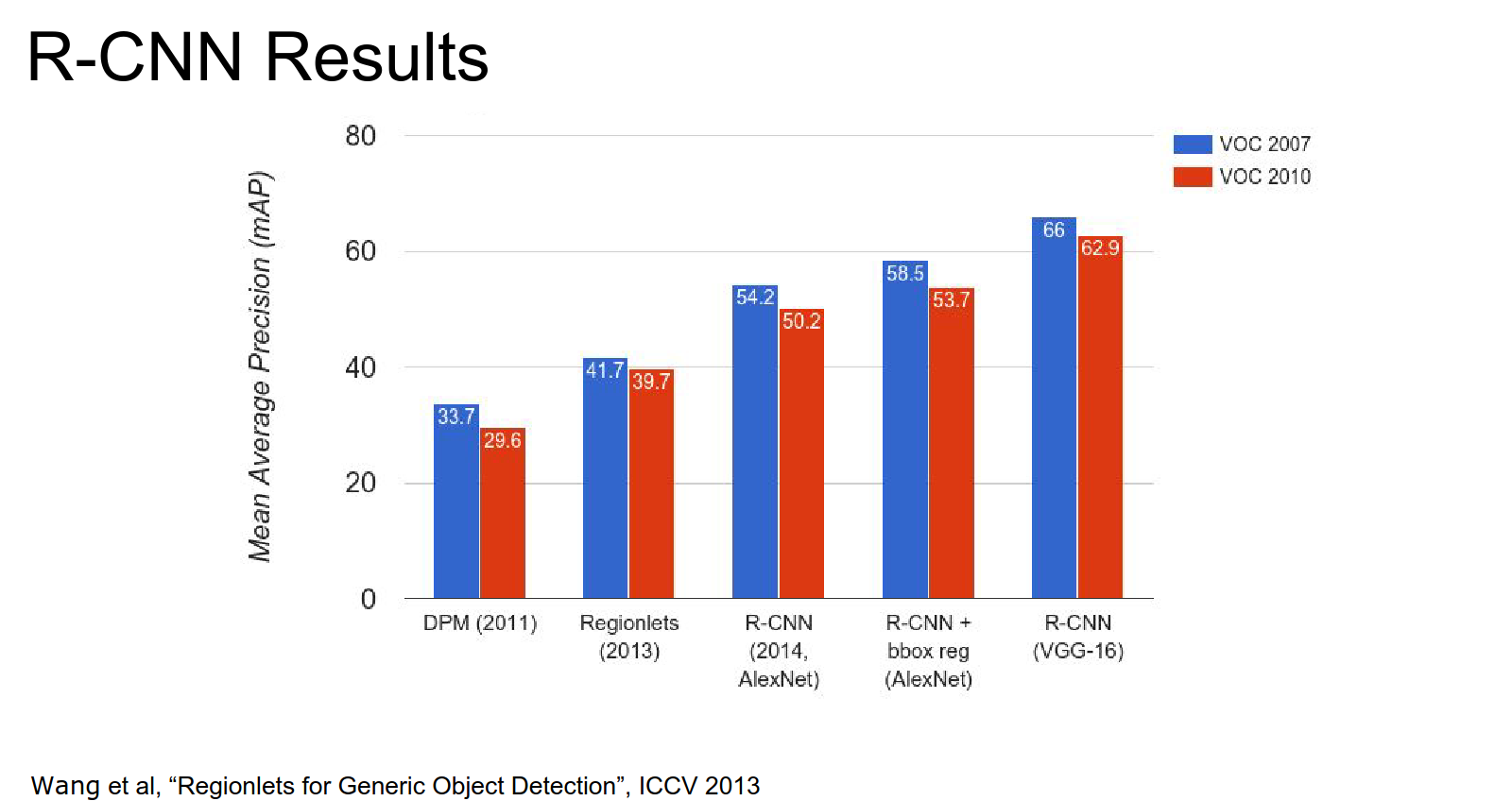
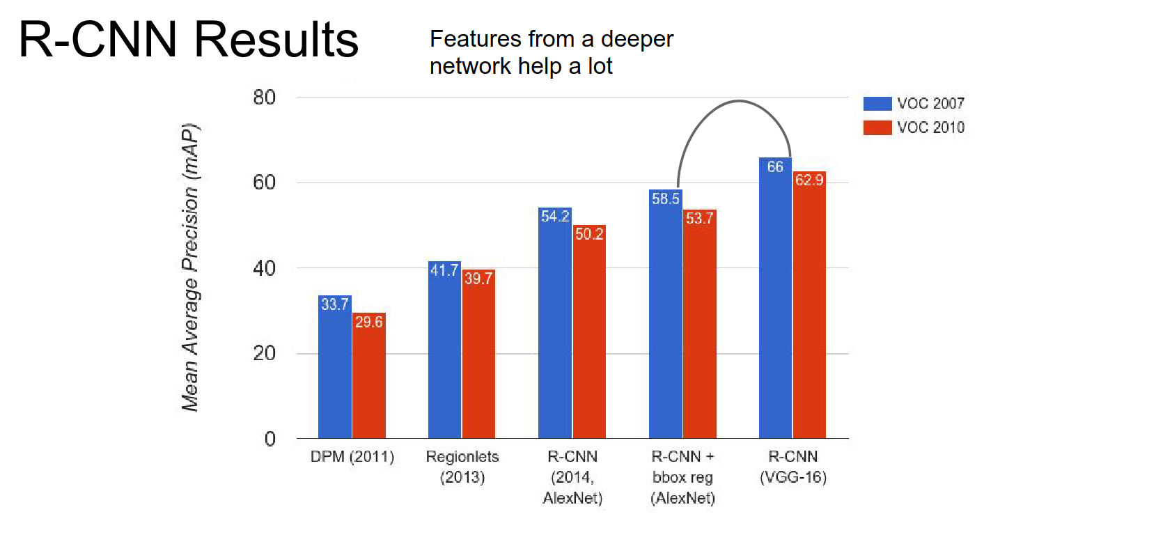
Pre-CNN vs. Post-CNN is a big improvement in terms of mAP.

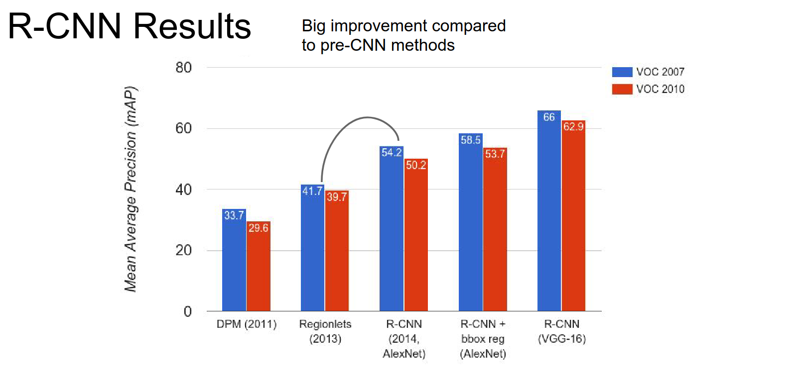
R-CNN has different results for AlexNet, bbox reg + AlexNet, and VGG-16.

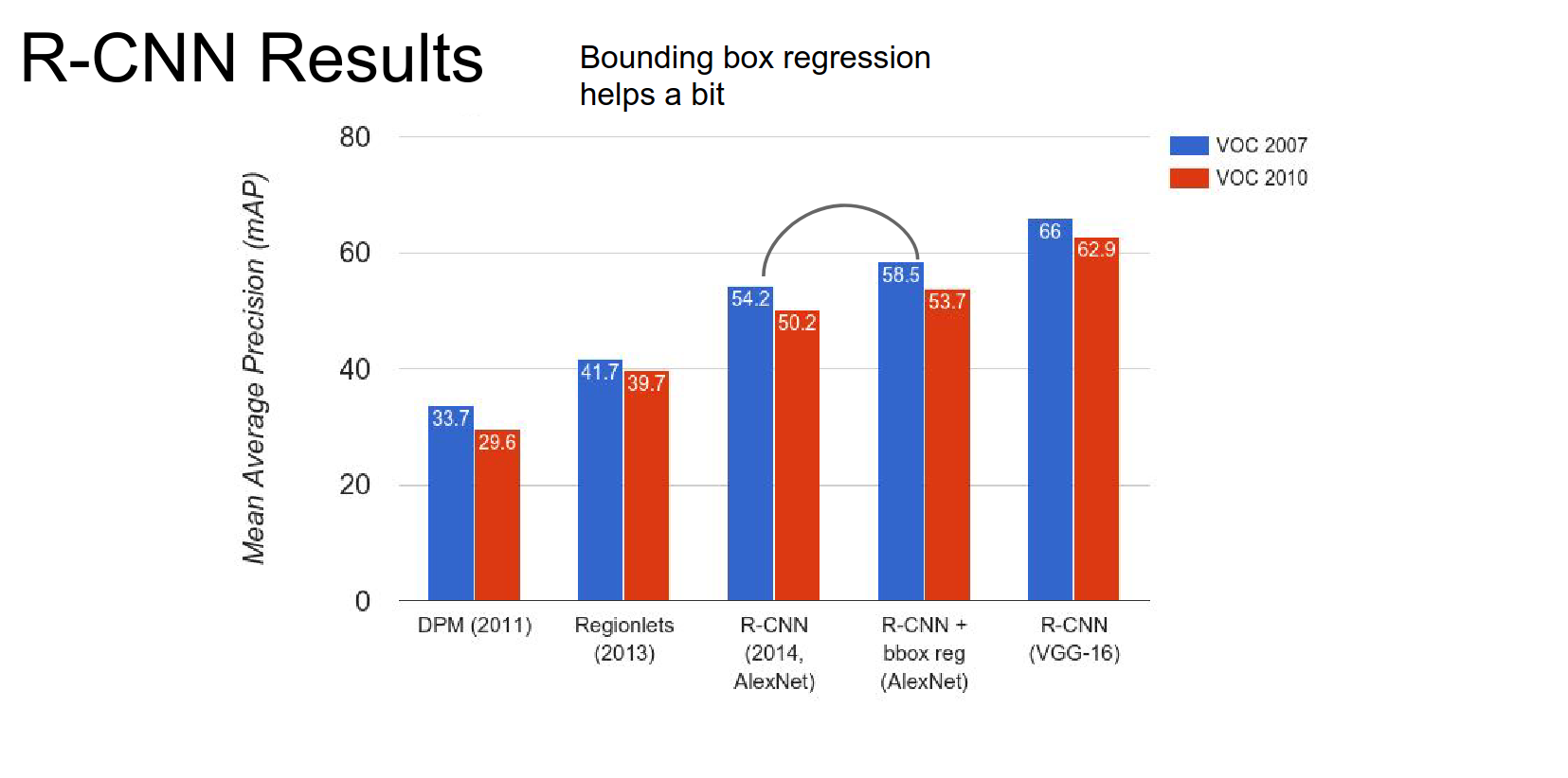
Features from deeper networks help a lot.

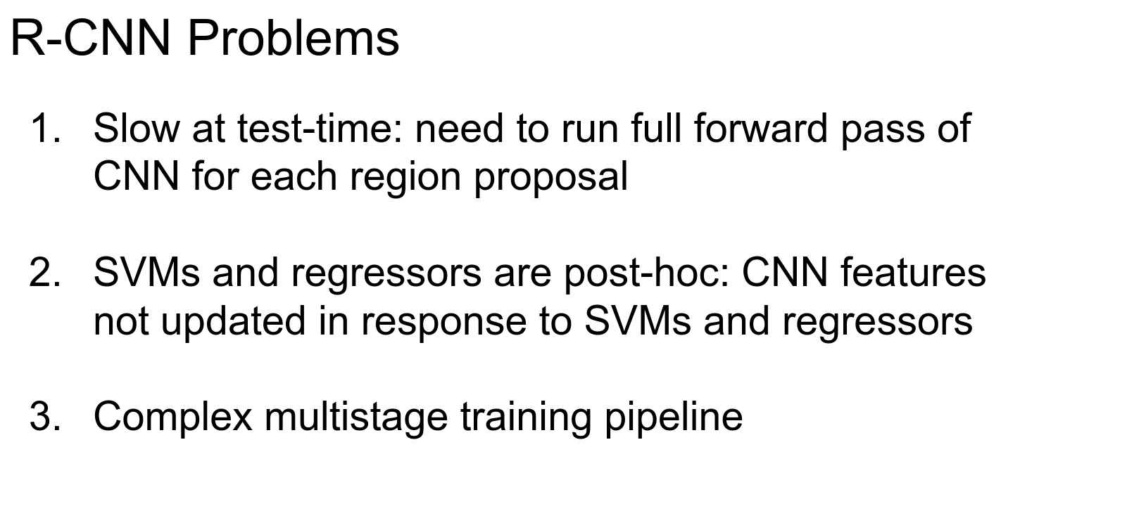
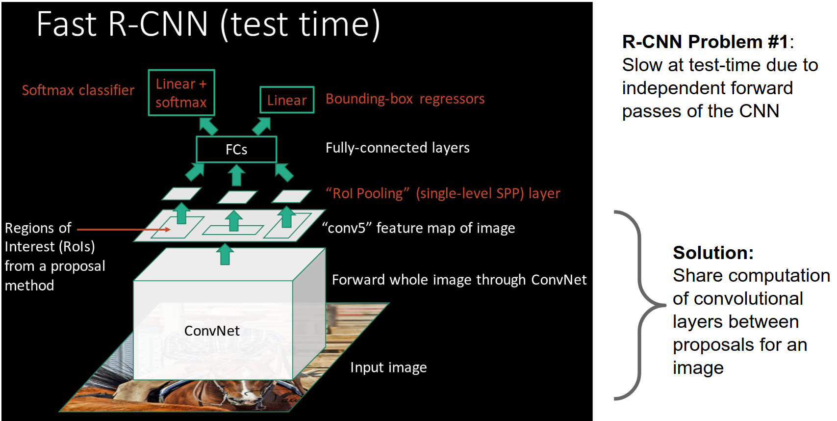
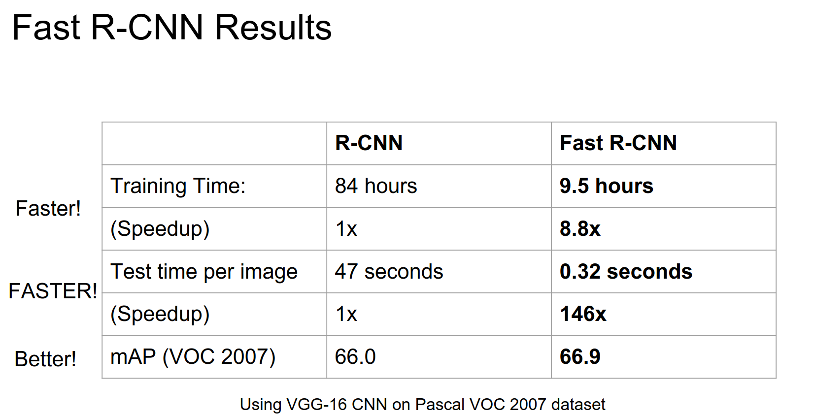
R-CNN is pretty slow at test time.

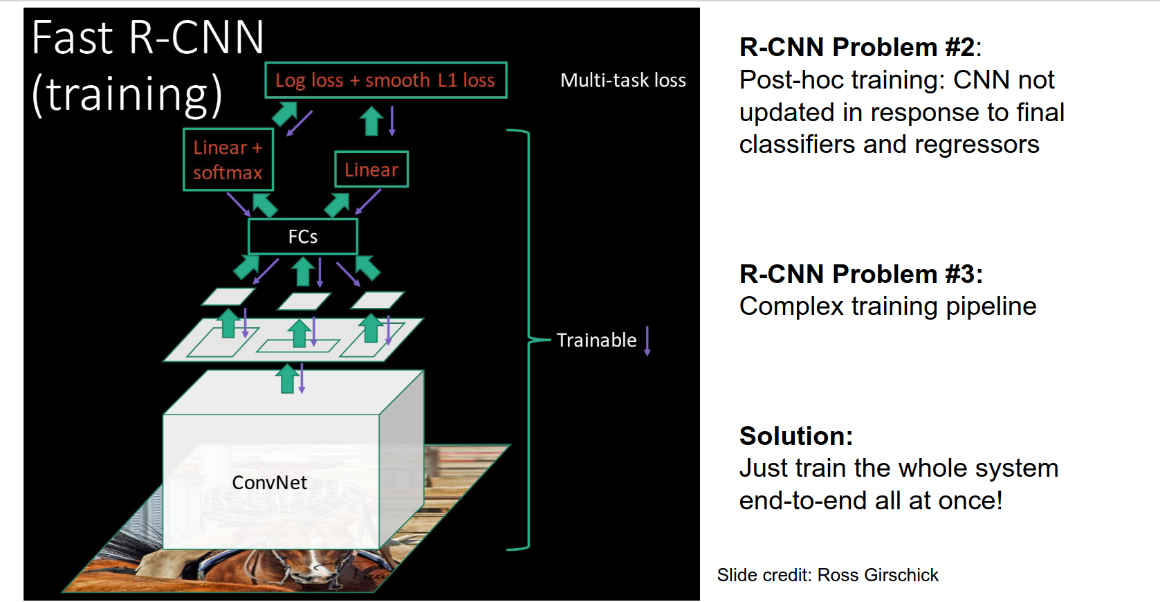
Our SVM and regression are trained offline. The CNN did not have a chance to update.

It's a complex multistage training pipeline.

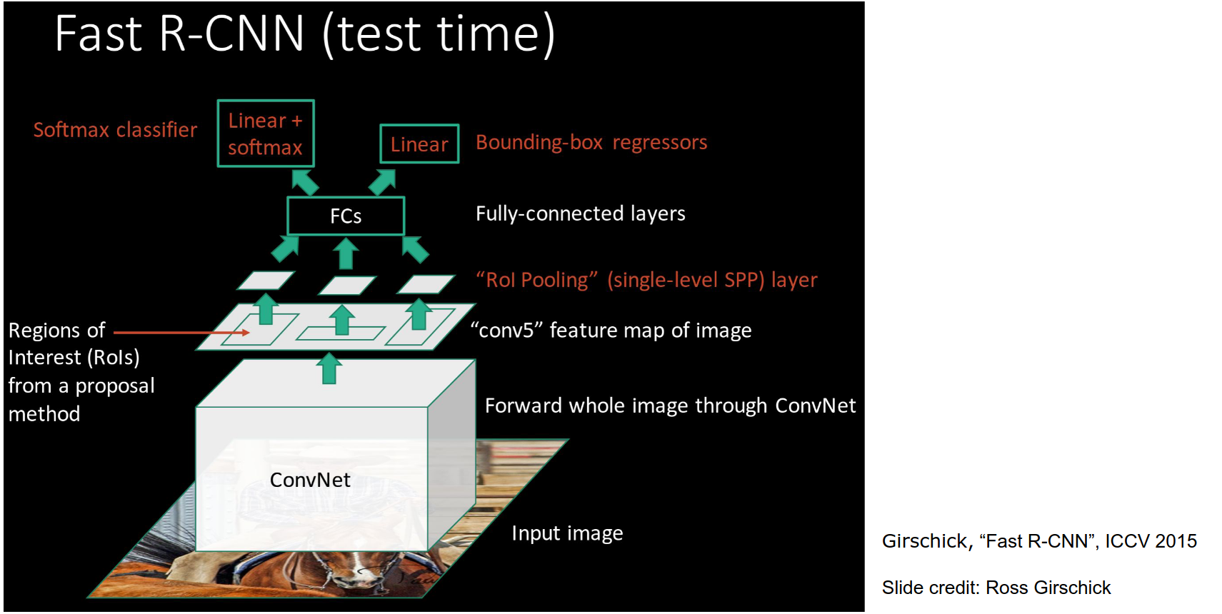
Fast R-CNN

• We are just going to swap the order of running a CNN and extracting regions.

Pipeline at test time:

• Take the high-res image.
• Run CNN - get a high-resolution Convolutional feature map.
• We will extract region proposals directly from this convolutional feature map using ROI pooling.
• The convolutional features will be fed to the fully connected layers and classification and regression heads.

Computation Sharing

Simplified Pipeline

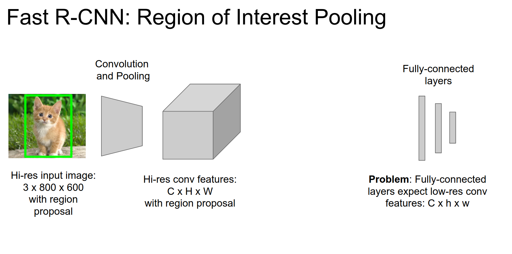
ROI Pooling 🤔

We have the input image in high resolution, and we have this region proposal coming out of selective search or edgeboxes.

We can put this image through convolution and pooling layers fine; those are scale-invariant.

Problem: FC layers are expecting low-res conv features.

Given a region proposal, we are going to project onto the spatial part of that convolution feature volume.

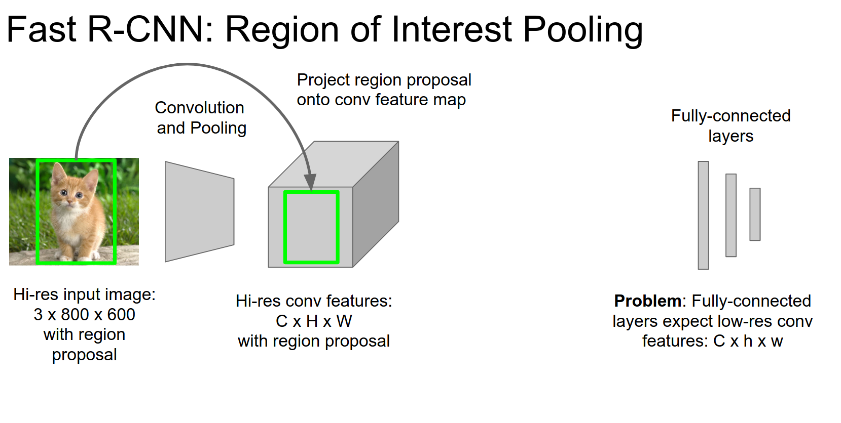
We will divide that feature volume into a grid.

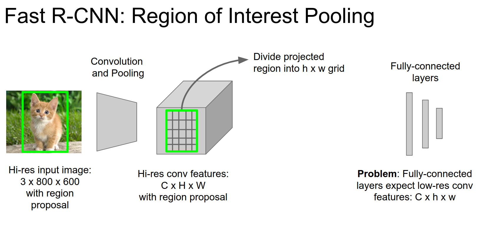
We do max pooling.

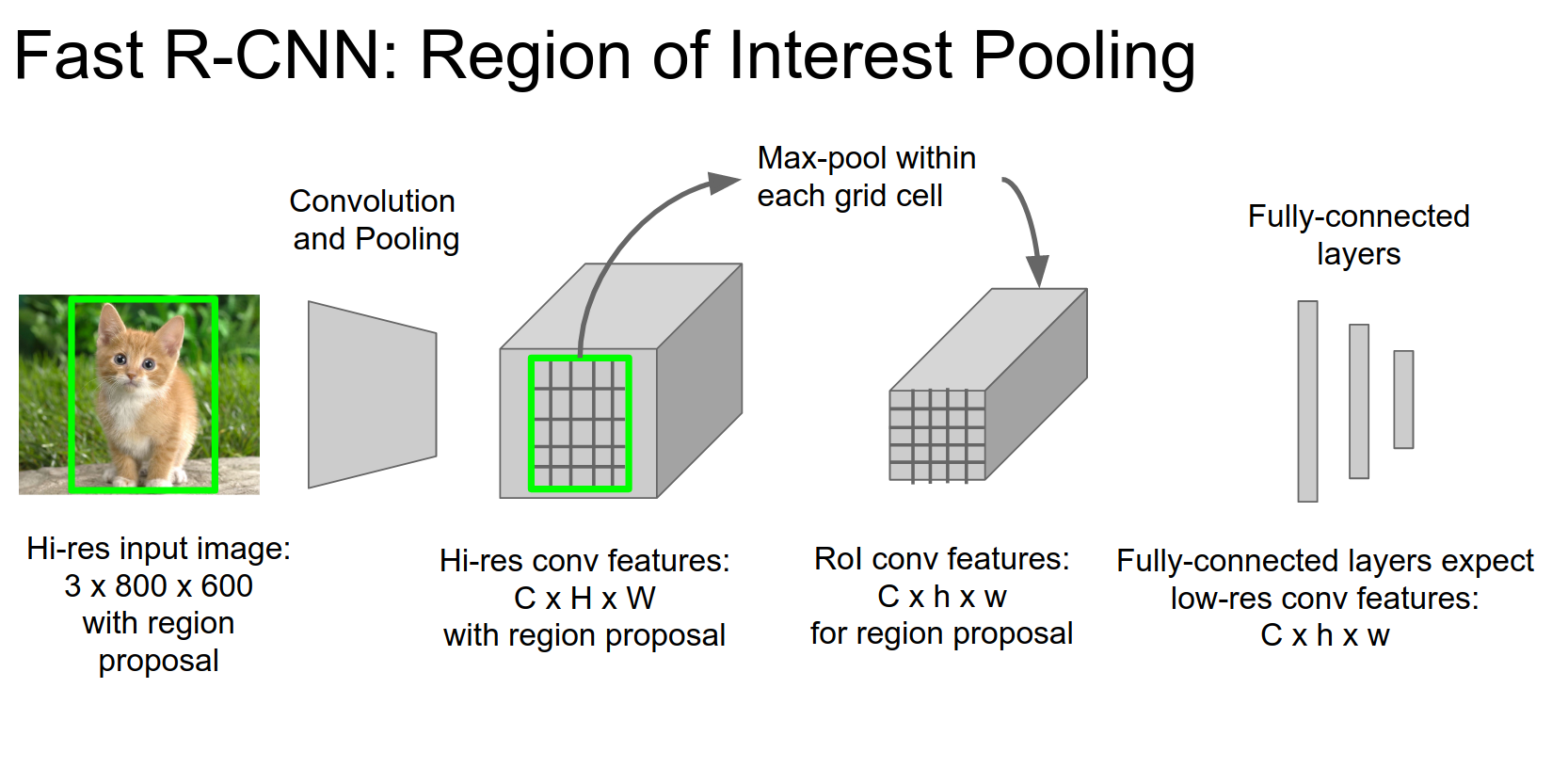
We have taken this region proposal, shared convolutional features, and extracted a fixed-sized output for that region proposal.

Optimization Tip: Swapping the order of convolution and wrapping and cropping.

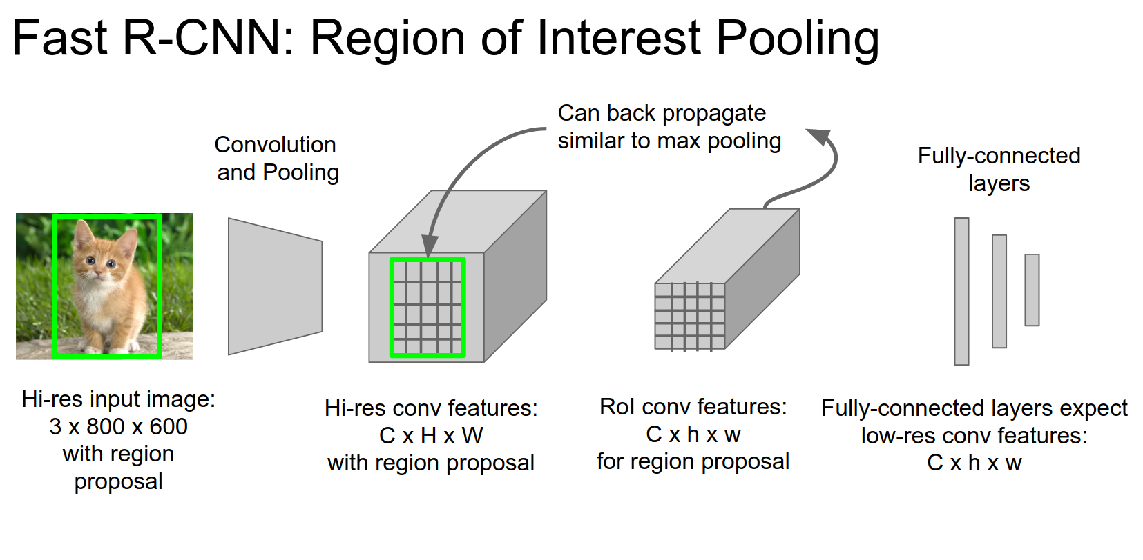
We can backpropagate from these regions of interest.

Joint Training

Now we can train this thing in a joint way!

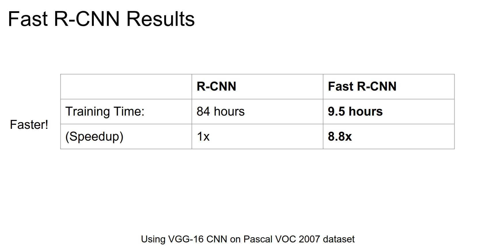
Much faster! 🐍

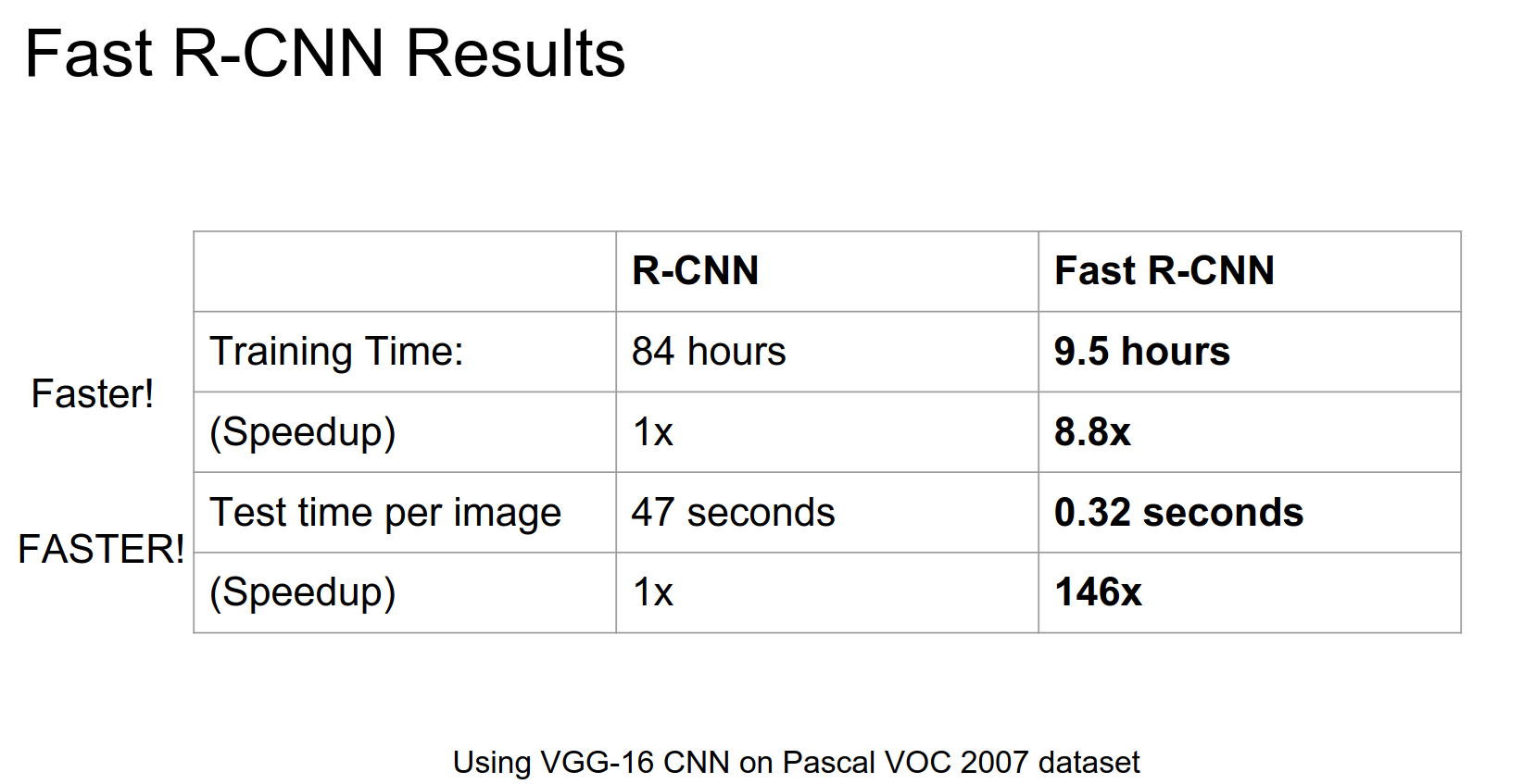
Test time shows huge improvements.

Not a huge improvement in performance, but solid.

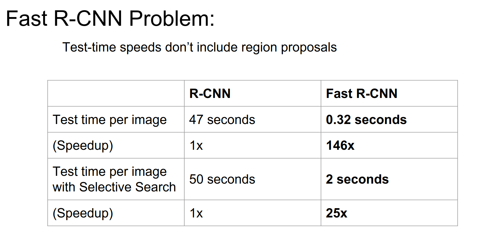
Bottleneck

This is still not Real Time.

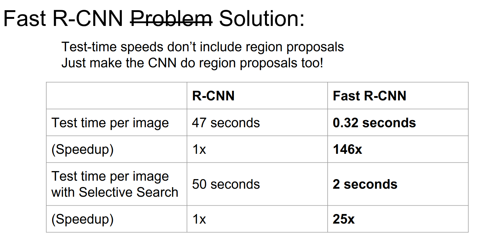
Faster R-CNN

Instead of using some external method, use a network.

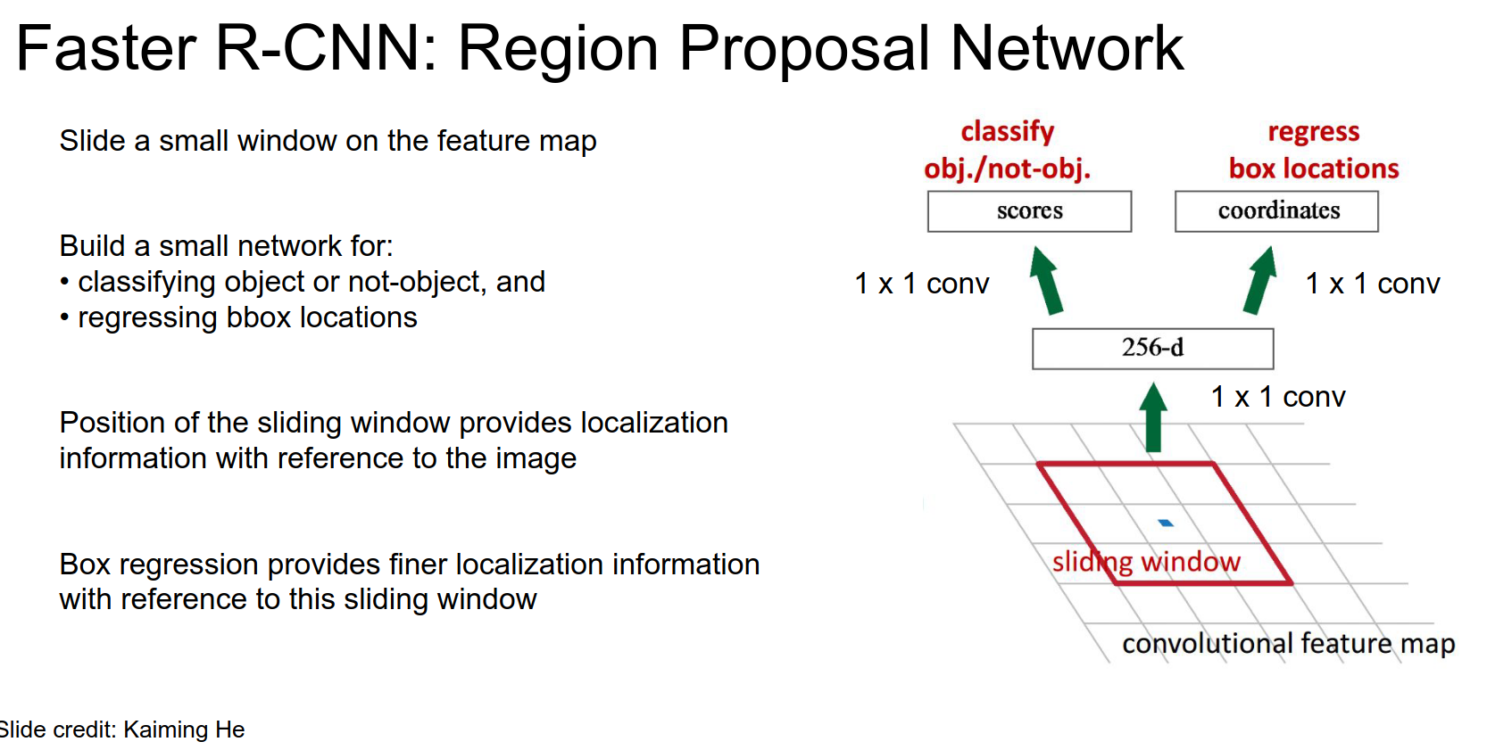
Region Proposal Network

RPN is trained for region proposal. It looks at the last layer's convolutional features and produces region proposals from the convolutional feature map.

After that, run just like Fast R-CNN.

How does it work?

We receive a convolutional feature map as input, coming out of the last layer. RPN is a CNN.

RPN Convolutions

Sliding window is a convolution.

• We are doing classification. Is there an object?

• Regression. Regress from this position to an actual region proposal.

The position of the sliding window relative to the feature map tells us where we are in the image.

Regression outputs give us corrections on top of the position on the feature map.

It's a little more complicated than that.

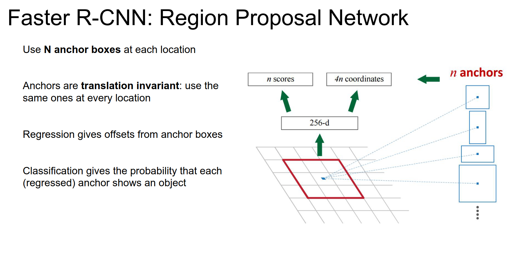
Anchor Boxes

Taking different sized and shaped anchor boxes and pasting them in the original image at the point corresponding to this point in the feature map.

Every anchor box is associated with a score and a bounding box.

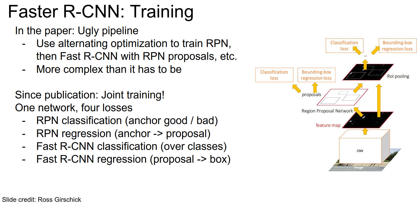
In the original paper, training was ugly. Since then, they had some unpublished work where they train this jointly.

They have one big network. In RPN, they have BB regressions and classification loss. They do ROI pooling and do Fast R-CNN.

• We get classification loss on which class it is, and regression loss for correction on top of the region proposal.

Loss Functions 🐦 🐦 🐦 🐦

Why not run convolutions on where we want? That is simply external region proposal tactic. We are better of making them with convolutions too because they became the bottleneck.

Rationale

RPN is a computational saving.

Now we can do object detection all at once. We are not bottlenecked anymore.

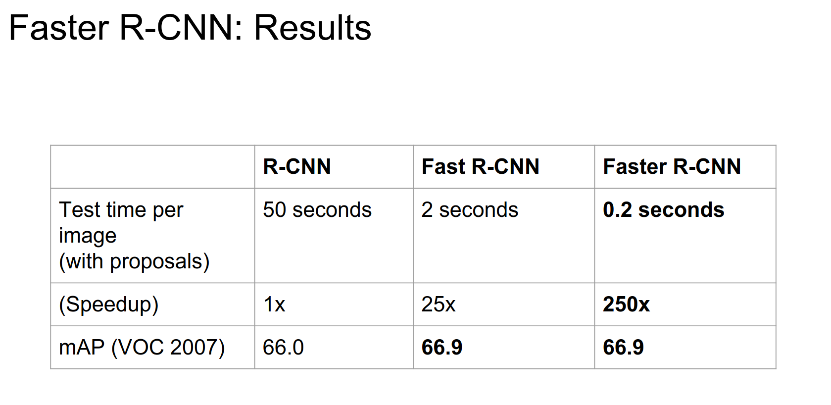
0.2s is pretty cool.

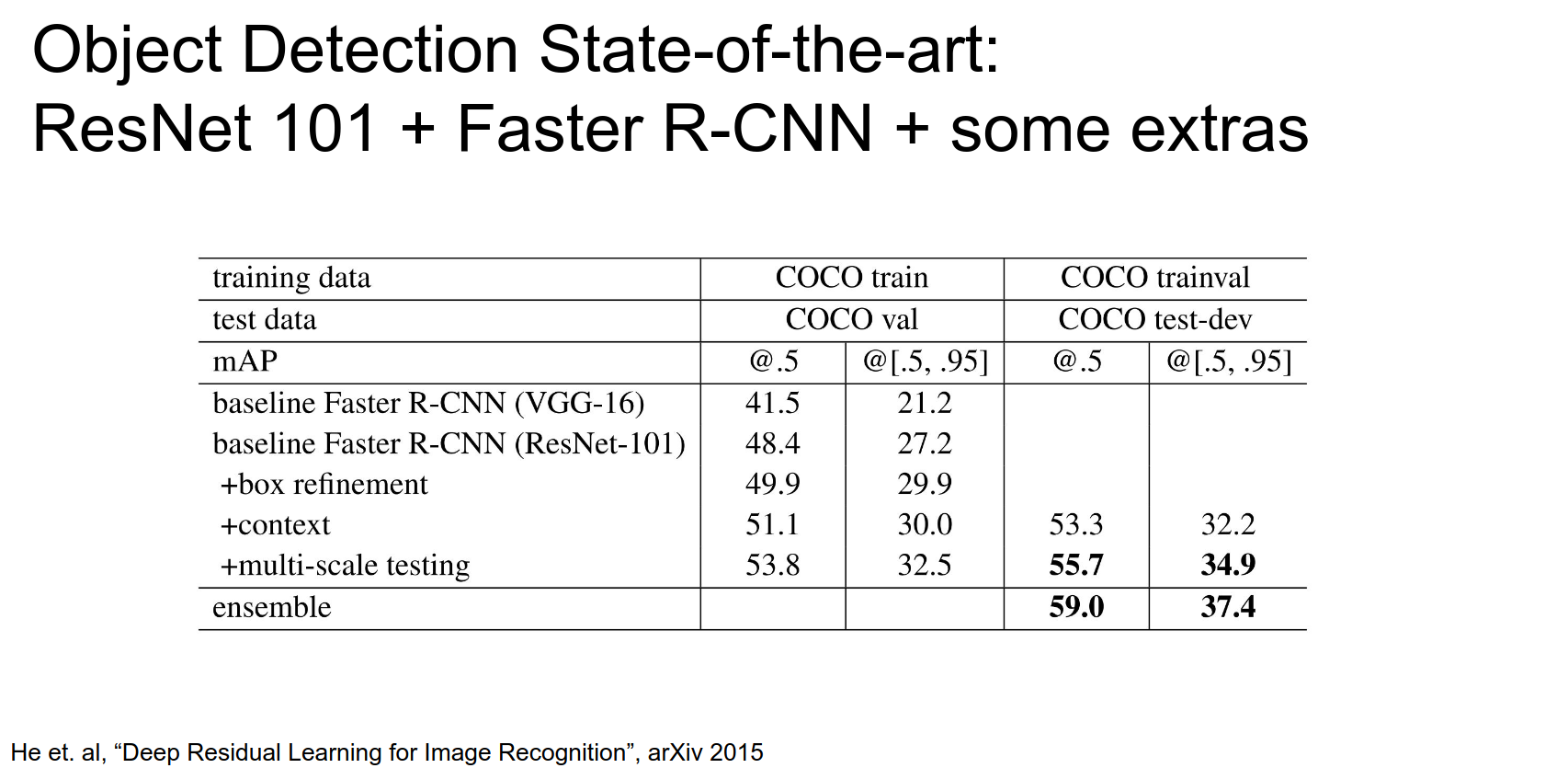
This is the best object detector in the world (in 2016).

ResNet Integration

Fancy stuff for competition:

• Box refinement: They do multiple steps for refining the bbox. You saw in the Fast R-CNN framework you are doing that correction on top of your Region Proposal; you can feed that back into the network to re-classify and get another prediction.

• Context: In addition to classifying just the image, they get a vector that gives you features on the entire image.

• Multi-scale testing: Kinda like OverFeat, they run the thing on different-sized images.

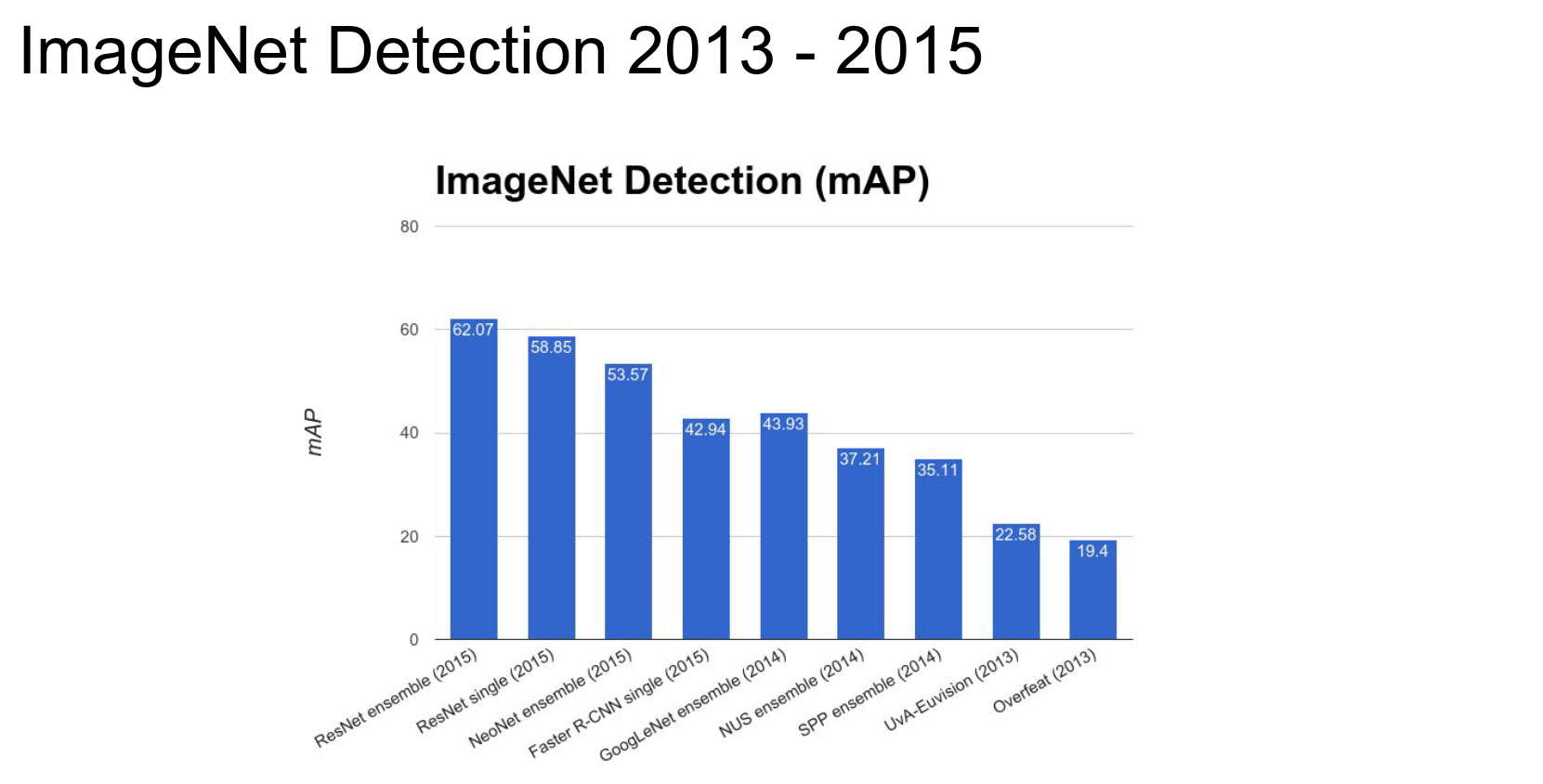
In 2013, Deep Learning Detection methods entered the arena.

After 2014, it is all about Deep Learning.

YOLO

Pose the detection problem directly as a regression problem.

• Divide image into grids.
• Predict B bbox - single score for that bbox.
• Now detection is a regression.

It is incredibly fast, but performance is lower.

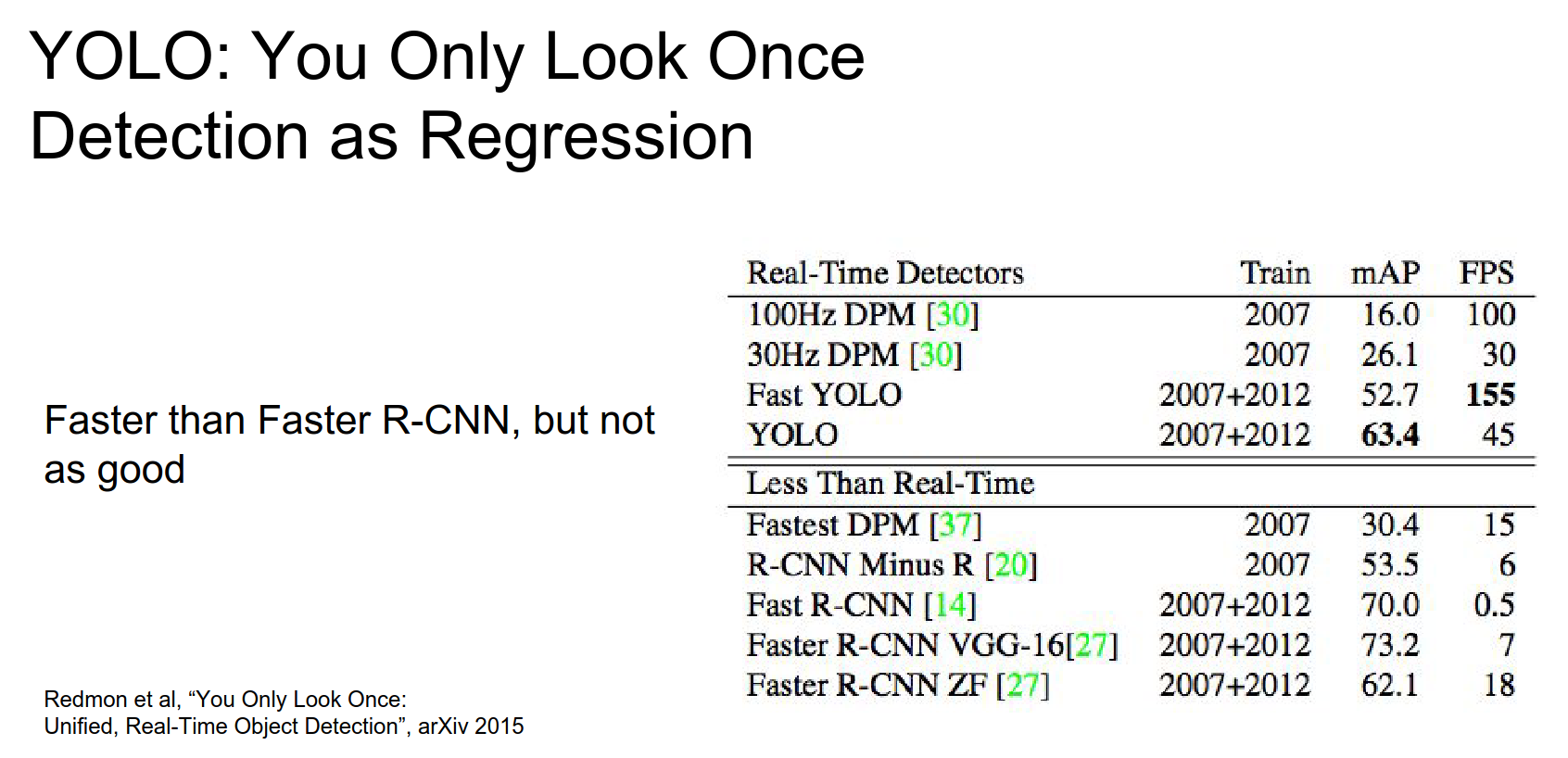
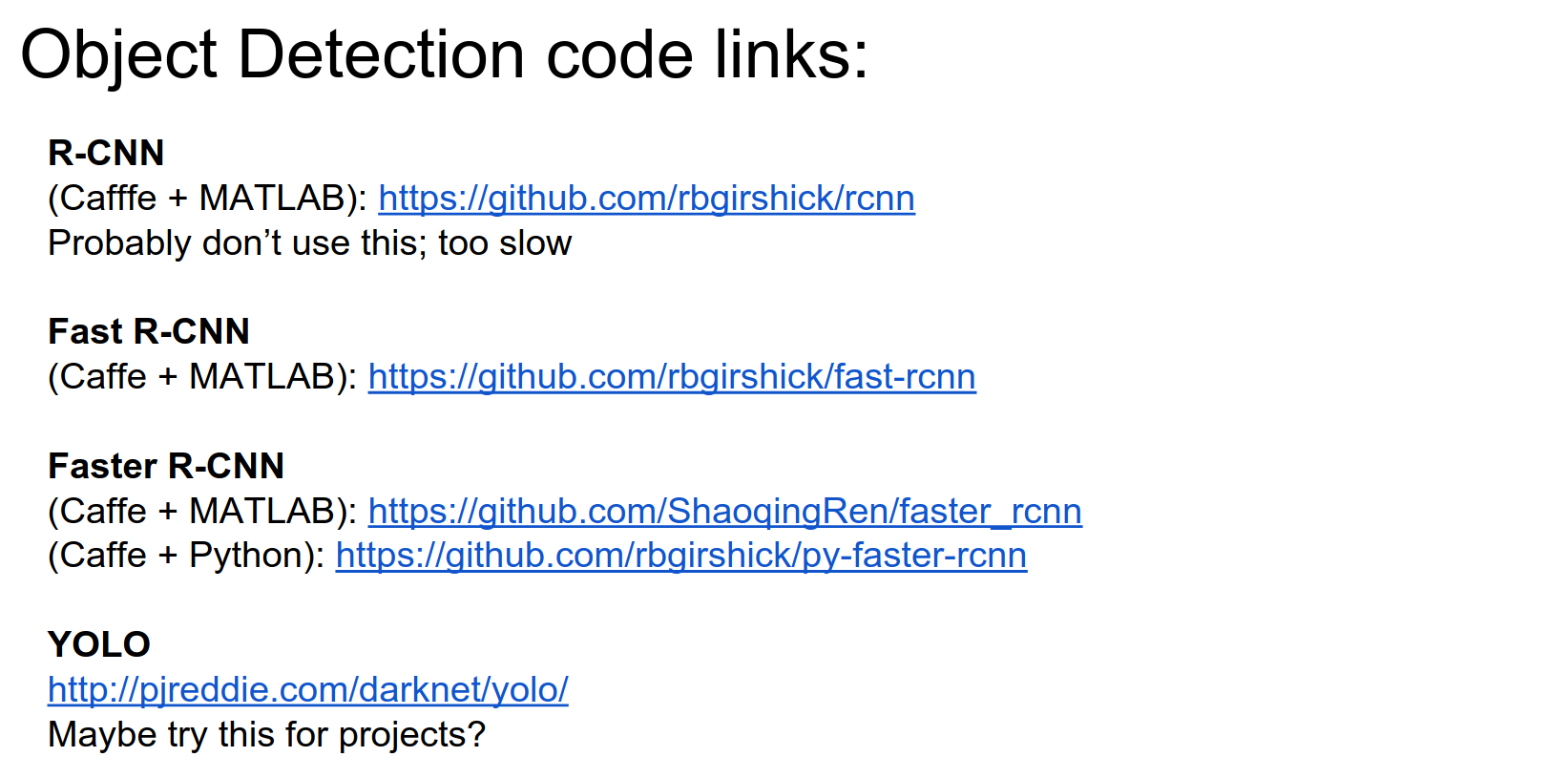
R-CNN: too slow. Fast R-CNN: requires Matlab. Faster R-CNN: might be good. YOLO: is solid.

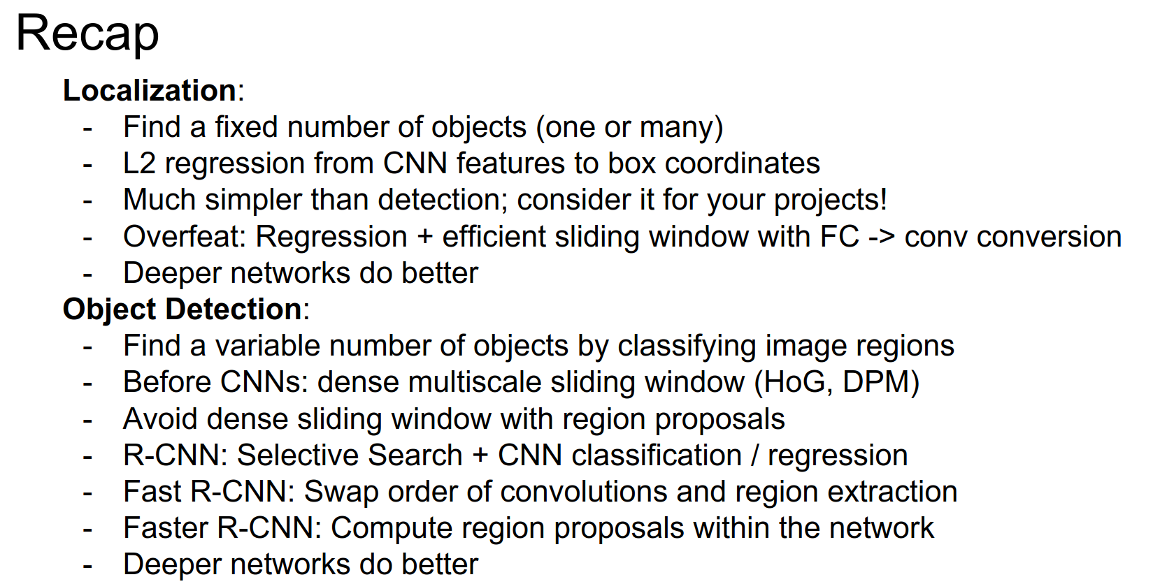
In localization, we are trying to find a fixed number of objects. This is much simpler than detection. We use L2 regression from CNN features to box coordinates.

OverFeat: Regression + efficient sliding window with Fully Connected Layer -> Convolution conversion.

In detection, we are trying to find a varying number of objects. Before CNNs, we used different features and sliding windows. That was costly.

We went from R-CNN to Fast R-CNN to Faster R-CNN.

Deeper is better, with ResNets.

Done with lecture 8!