9. Understanding and visualizing ConvNets
Part of CS231n Winter 2016
Lecture 9: Understanding ConvNets
This is one of Andrej's favorite lectures to give.
Assignment 2 is almost due. The midterm is next week. They just released the winning weights.
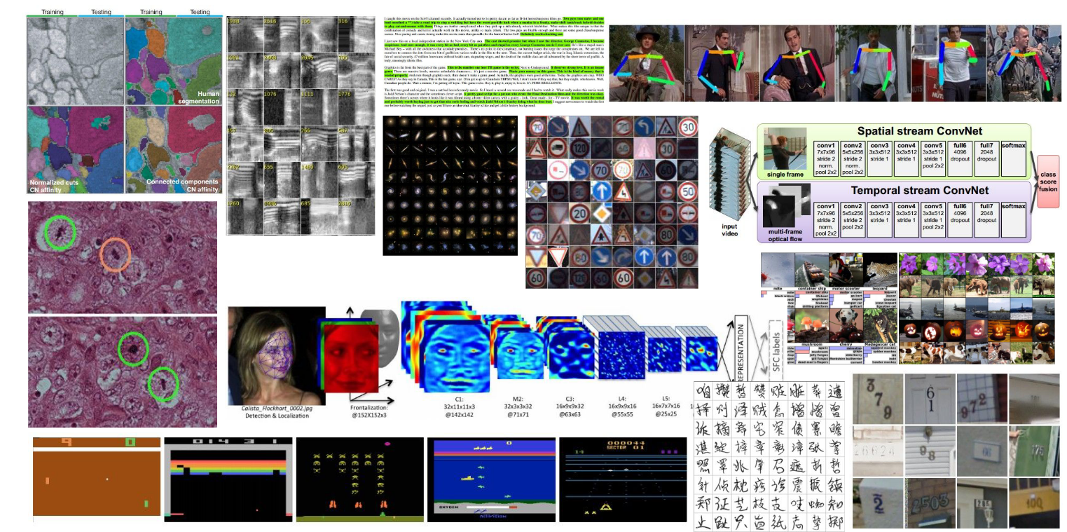
There is a wide variety of application domains for CNNs.
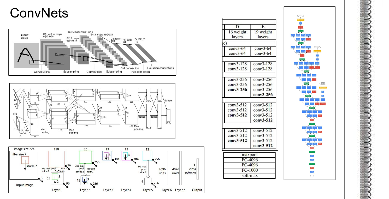
We saw how ConvNets work. We covered all the basics.
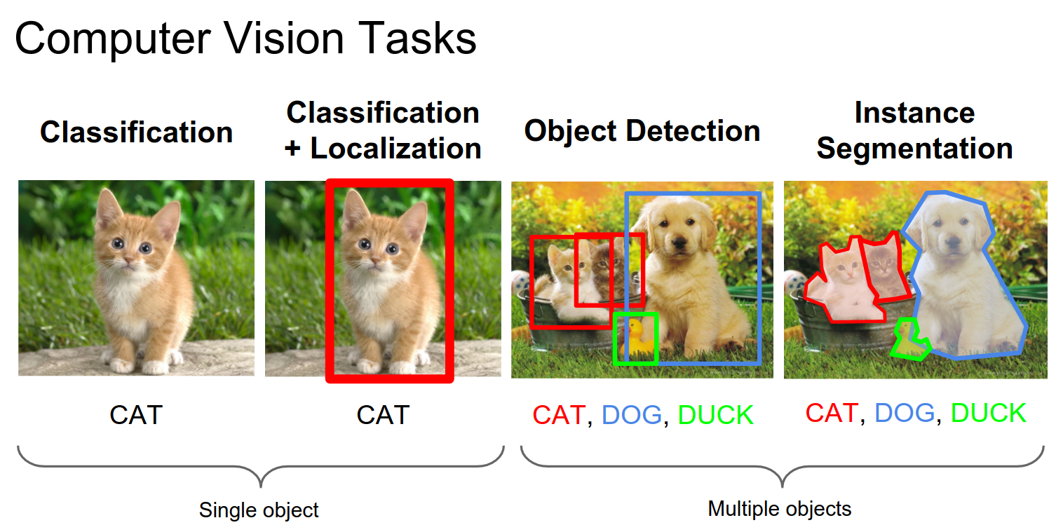
We looked at a lot of different Computer Vision tasks, including R-CNN, Fast R-CNN, Faster R-CNN, and YOLO.
Multiple heads are placed on top of a ConvNet; some heads do classification, and some do regression. They are all trying to solve the problem at hand.
Understanding ConvNets
We will go over all of these bullet points.
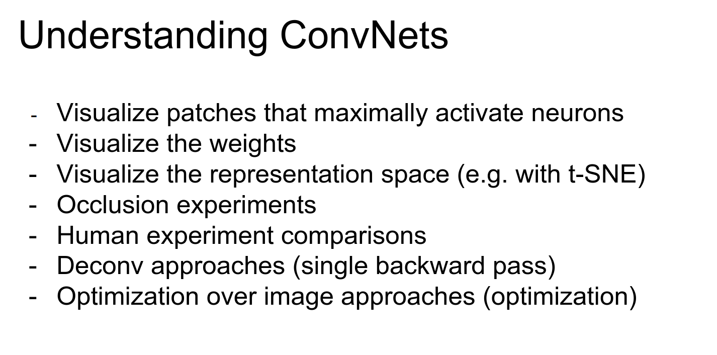
Perhaps the simplest way to understand what a ConvNet is doing is to look at its raw activations.
In a CNN, we pass an image into the bottom, and we get activation volumes in between.
We can select a random neuron—say, on the pool 5 layer—pipe a lot of images into the ConvNet, and see what excites that neuron the most.
Some of them like dogs, some like flags. Some like text, and some like lights.
Visualizing Weights
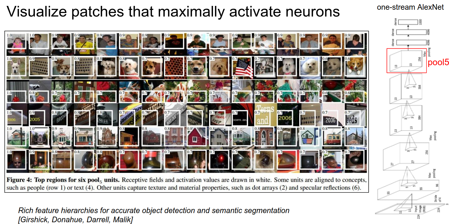
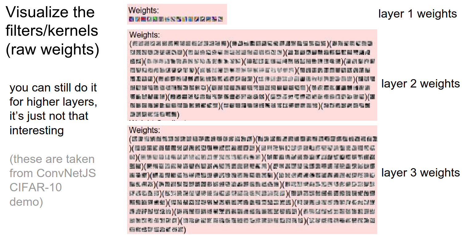
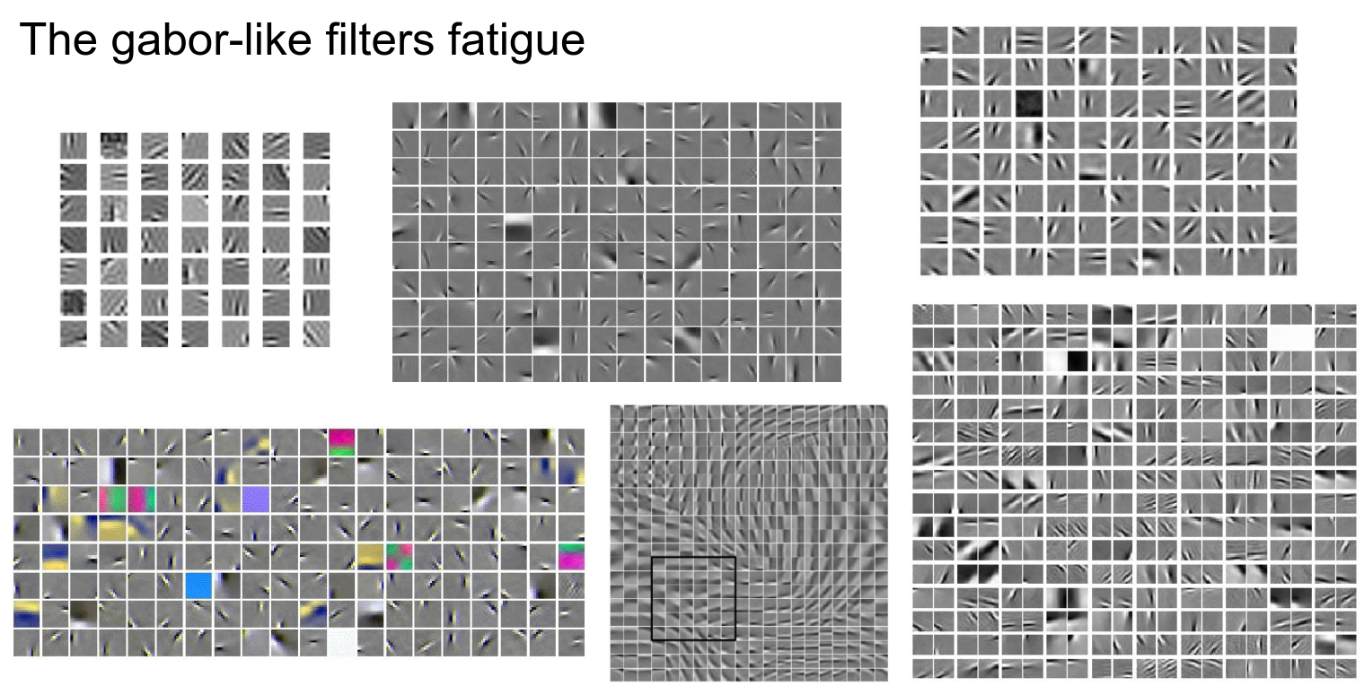
On the first layer, we can visualize the weights. In the first layer of convolution, we have a filter bank that we slide over the image, so we can visualize the raw filter weights.
When weights are not directly connected to the image, visualization doesn't really make sense. It only makes sense in the first layer.
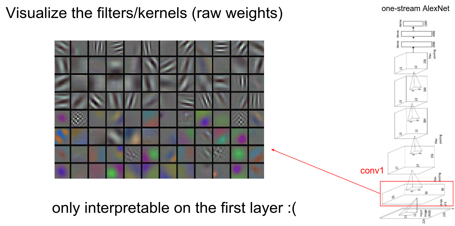
You can still do it, but it doesn't make as much sense.
Pretty much anything you throw at an image to learn a feature will result in these Gabor-like features (Gabor filters, a mathematical function used in signal processing), regardless of the algorithm.
The inverse is actually hard to do for the first layer. The example Andrej gave is PCA; it doesn't give Gabor-like features, but rather sinusoids.
Global Representation
We looked at filters and weights.
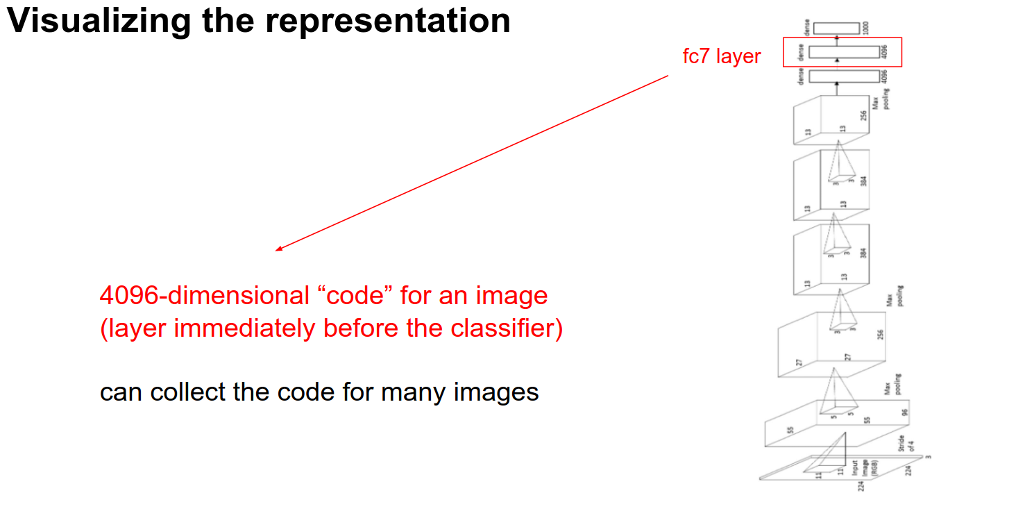
Another way to look at it is to pass a lot of images through the ConvNet and look at the FC-7 Features.
These are 4096 numbers just before the classifier. These numbers summarize the content of the image. These are codes we can use.
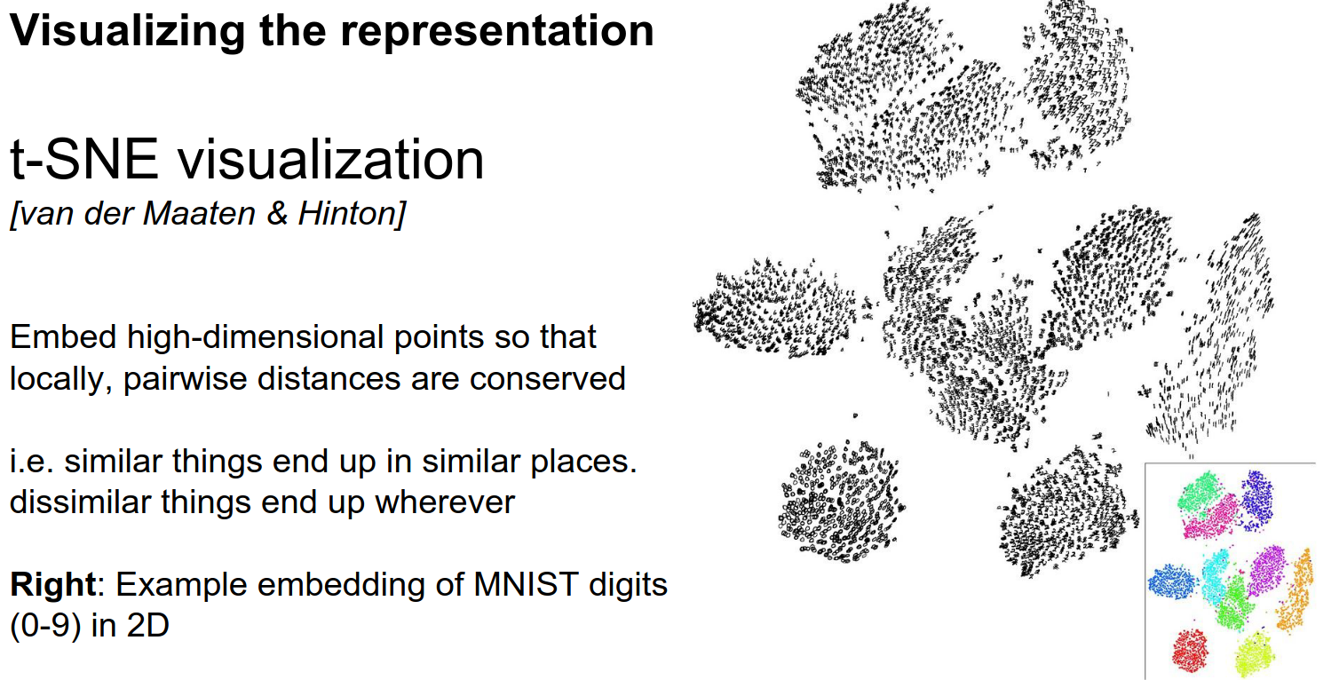
t-SNE Visualization
You give it a collection of high-dimensional vectors, and it finds an embedding in 2D such that points that are nearby in the original space are nearby in the embedding.
It does this in a clever way that gives us really nice-looking pictures.
Below you can see the embeddings for MNIST:
Embedding Proximity 🍉
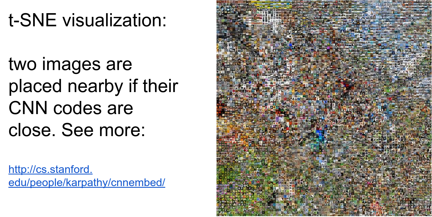
Here is the link, and the full image is below. All the boats are close, all the spaghetti is close, as are all the dogs and animals.
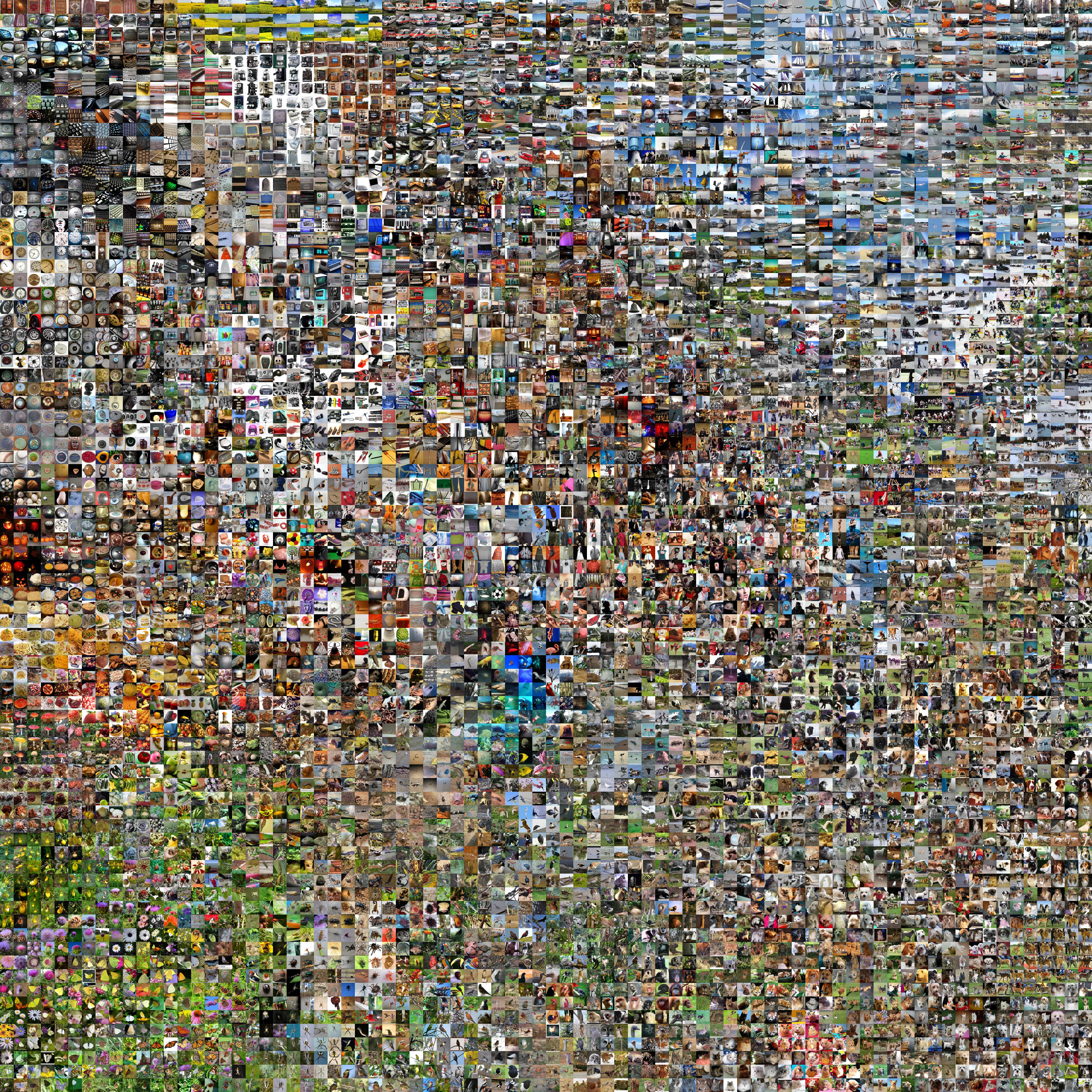
This is what ConvNets consider similar.
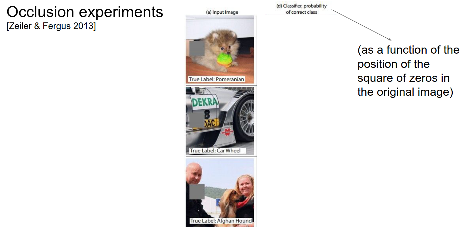
Occlusion Experiments 🐔
Visualizing and Understanding Convolutional Networks by Matthew D. Zeiler and Rob Fergus, published in 2013.
The main idea behind occlusion experiments is to understand which parts of an input image are crucial for a CNN's decision-making process. This is achieved by systematically occluding (covering) different parts of the input image and observing how the network's output changes as a result.
-
A patch of zeros (occluder) is shown in grey.
-
We slide it over the image.
-
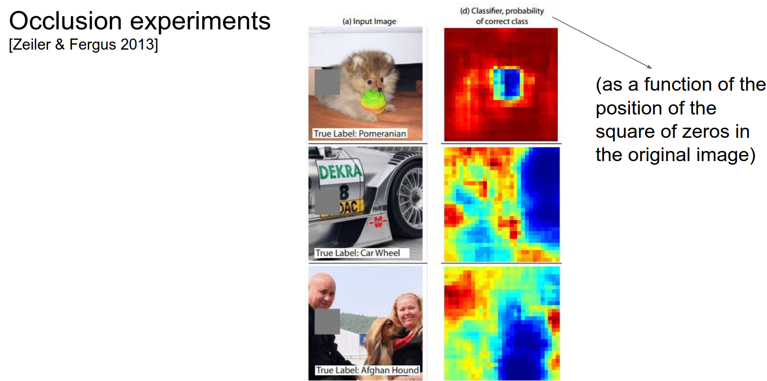
As we do that, we look at the probability of the class and how it varies as a function of the spatial location of that occluder.
We would expect the probability to go down when we cover up the dog. That is basically what happens.
We get a kind of heat map from this.
The same applies to the dog and the car wheel.
In the last picture, interestingly, when you cover the person on the left, the probability goes up!
This is because the ConvNet is not sure if the class is there or not. When you remove the person, the ConvNet becomes more sure.
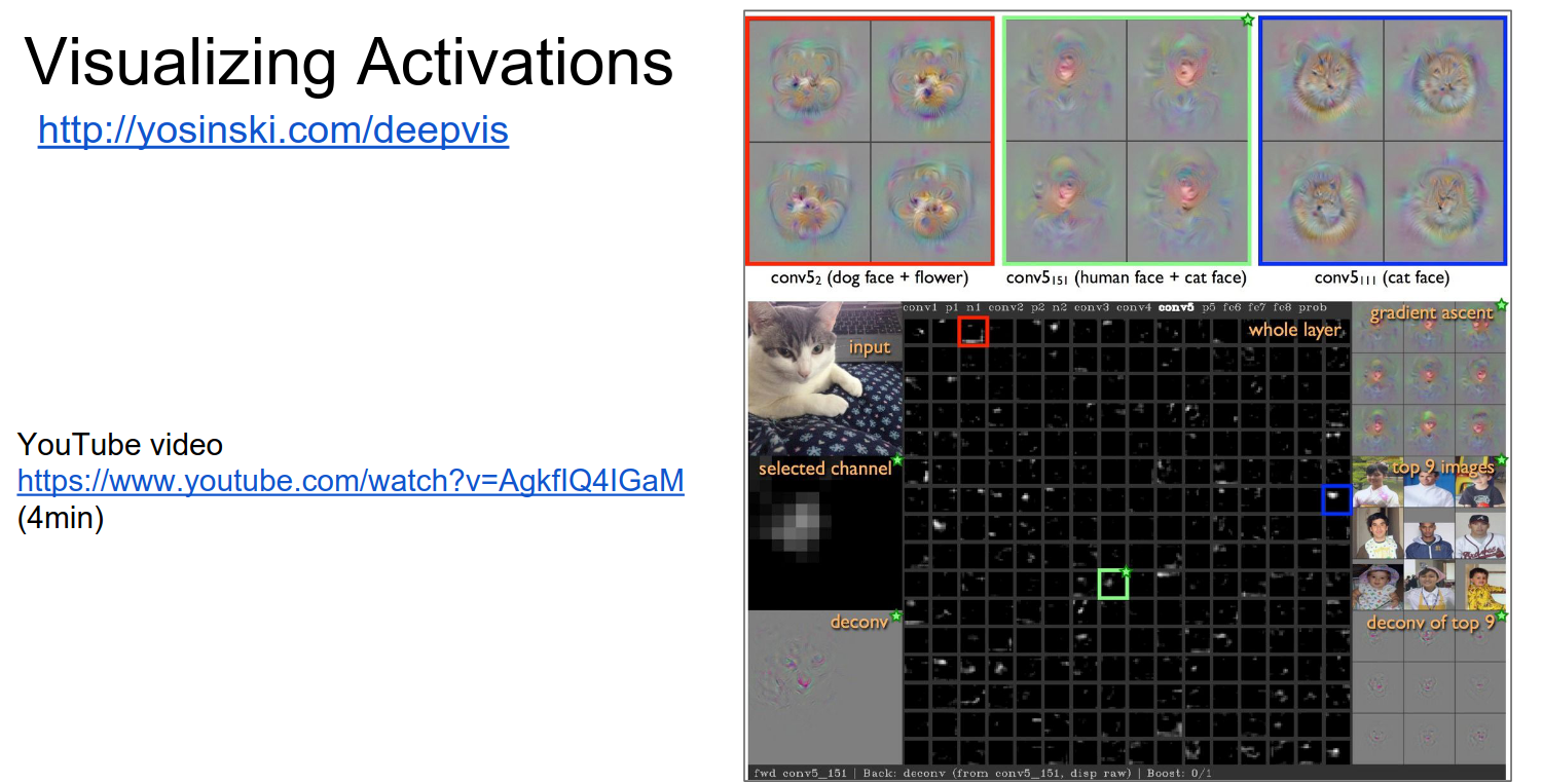
DeepVis Toolbox
Jason Yosinski! Running a ConvNet in real-time, you can summon your camera feed and play with the ConvNet to see all the activations.
2 Methods:
- Deconvolution
- Optimization Based
Watching the video!
Neural Networks are really good at classification, thanks to Convolutional Neural Networks.
Conv Layer 1: Light to dark or dark to light; different layers like different things. Some layers like heads and shoulders and ignore the rest of the body.
Some layers activate when they see cats. Some activate on non-smooth (wrinkled) clothes (not the clothing itself). Some just like text.
You can investigate and debug ConvNets in real-time.
Deconv Approach
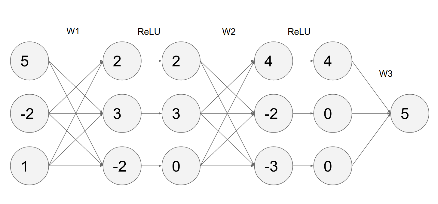
How would you compute the gradient of any neuron with respect to the image?
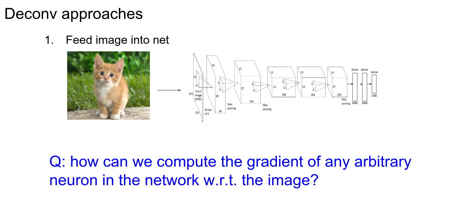
Normally, we have a computational graph, pass the image through, and get a loss at the end. We start with \(1.00\) in our computational graph because the gradient of loss with respect to loss is 1.
We want to backpropagate and find the influence of all the inputs on that output.
Gradient Computation 🤨
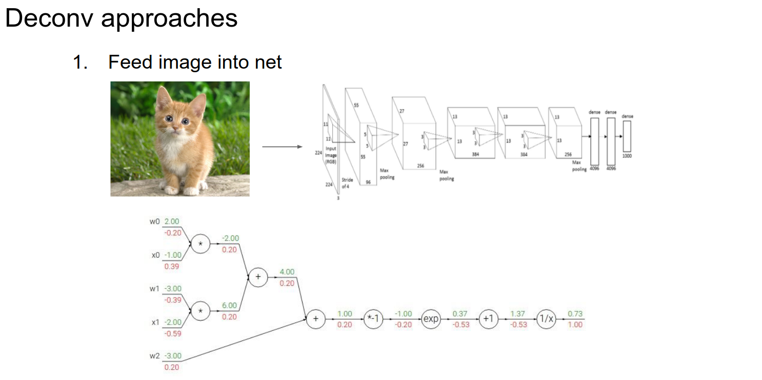
- We forward pass until some layer.
- We have activations for that layer.
- We are interested in some specific neuron.
- We zero out all the gradients in that layer except for the neuron's gradient we are interested in; we set that neuron's gradient to \(1.00\).
- Run backward from that point on (backpropagate).
- When you backpropagate to the image, you will find the gradient of the image with respect to any arbitrary neuron by playing with the gradients.
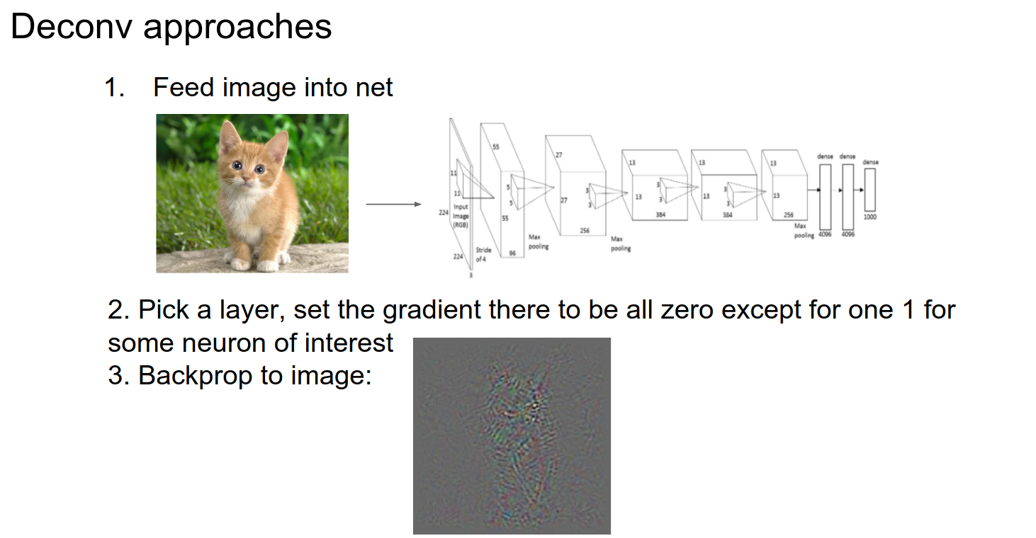
You will find something like this.
The Deconv approach changes the backward pass a bit; it's not entirely clear why.
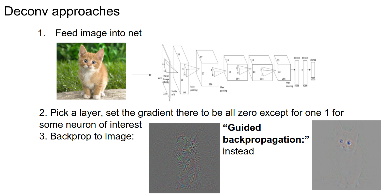
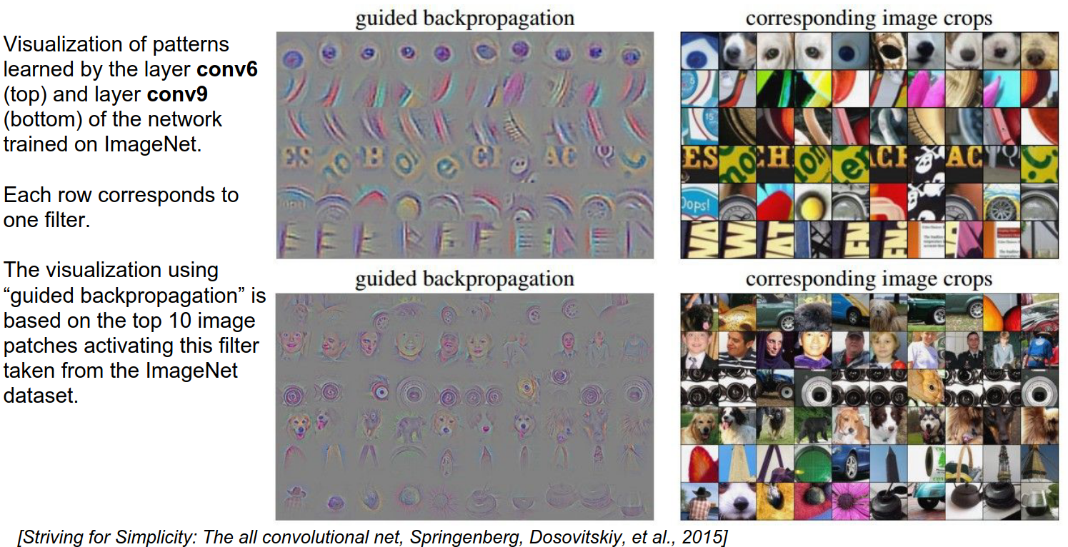
Guided Backpropagation
Much cleaner images, showing the cat's face.
This is a figure from the paper: The image goes through layers, and we get an activation map at some place.
We zero out all the gradients except the one we are interested in.
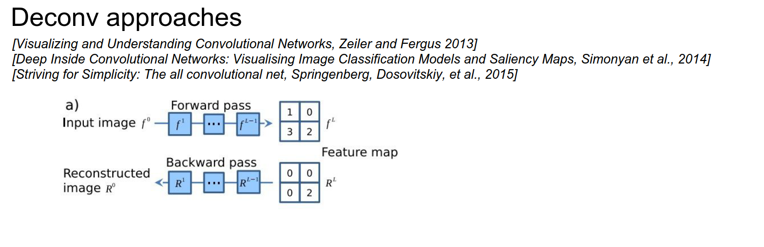
To get your Deconv to give you nice images, we will run backpropagation, but we will change the backprop in the ReLU layer!
You can see in c) that we have the activation, just like we described.
If your input was negative, you block the gradient in the backward pass, as per ReLU.
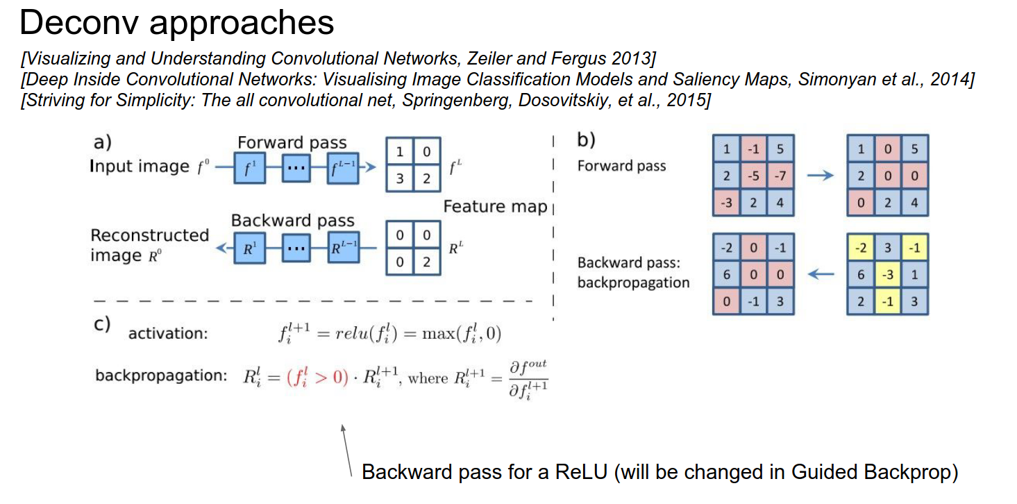
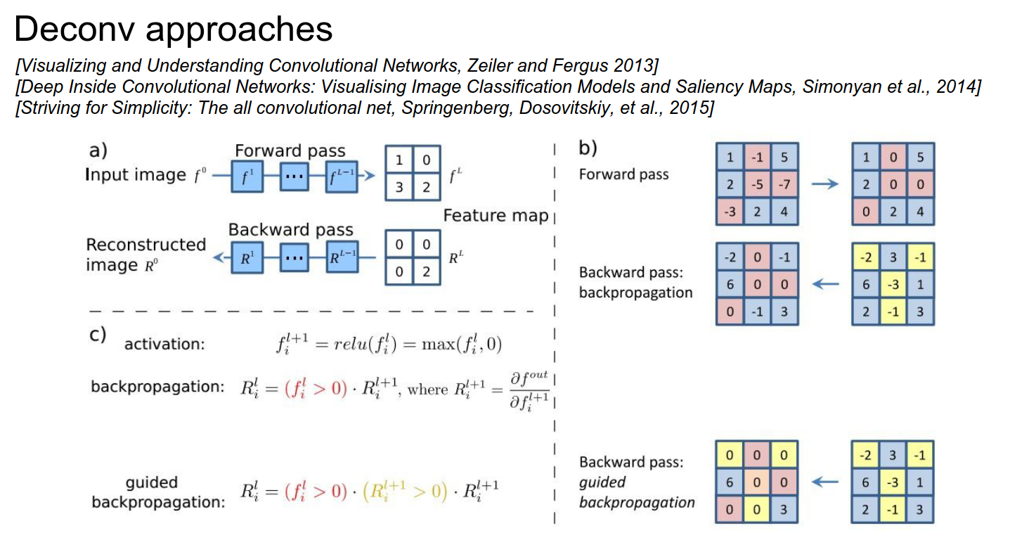
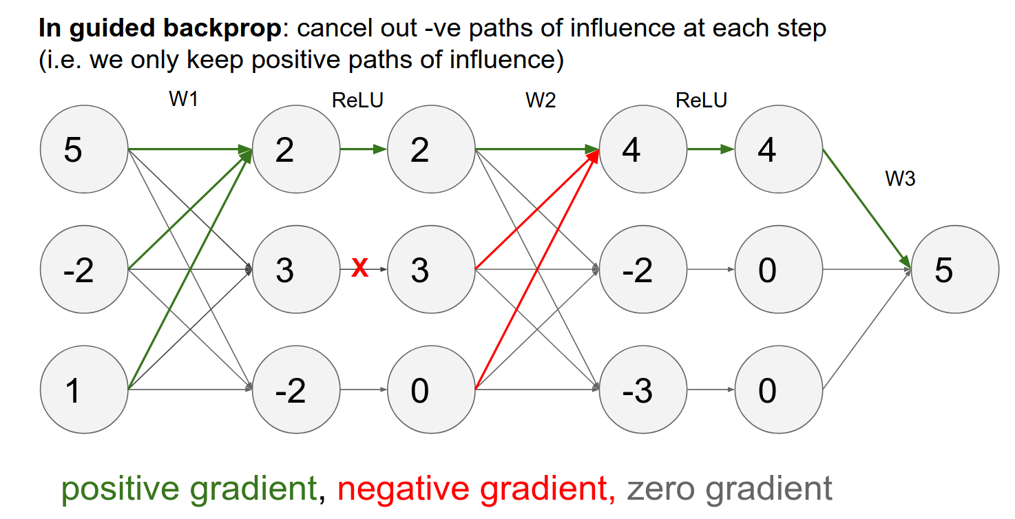
In guided backpropagation, we change the backward ReLU in the following way:
We compute what we had before, but we add a term that says we only backpropagate through our ReLU neurons where the ReLU neurons have a positive gradient.
Normally, we would pass any gradients corresponding to the ReLU neuron that had less than zero input. Now, in addition to that, we block out all the gradients corresponding to negative gradients.
Interpretation
- We are trying to compute the influence of the input on some arbitrary neuron in the ConvNet.
- A negative gradient means that the ReLU neuron has a negative influence on the neuron we are investigating.
- By doing that, we only pass through gradients that have an entirely positive influence on the activations.
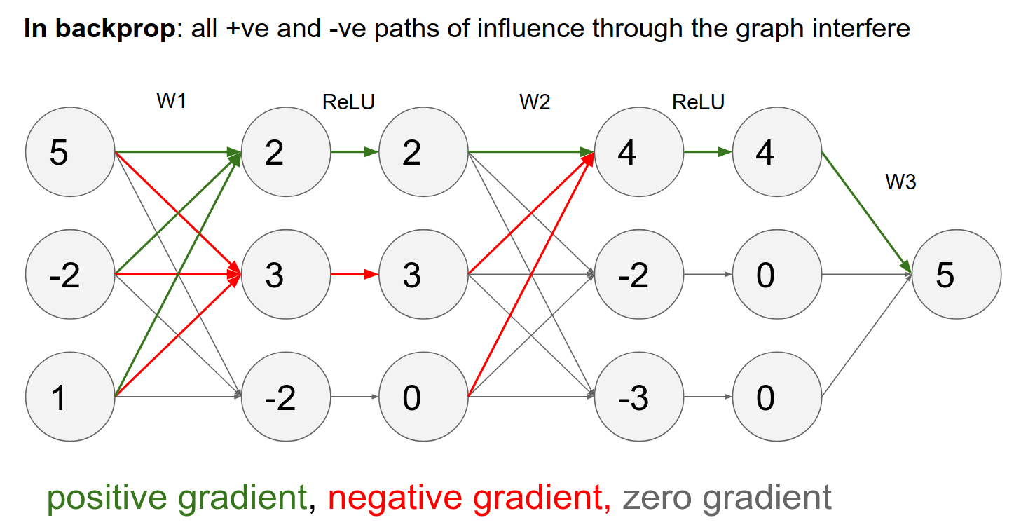
Backpropagation Dynamics
The reason we get weird images (like the one with the cat) is that some influences are positive and some are negative from every single pixel to the neuron we are investigating.
In guided backpropagation, we only use positive influences—only the positive gradients from the ReLU.
You get much cleaner images.
Another approach is DeconvNet:
- It ignores the ReLU gradient.
- It just passes through the positive gradient; it does not care if the activations coming to the ReLU are positive or negative.
- It works well.
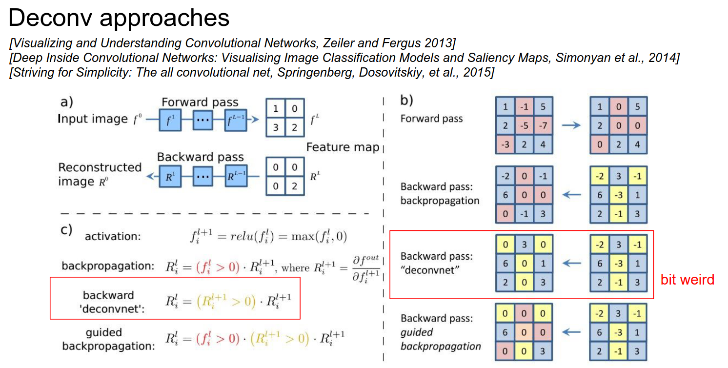
This is a similar idea to guided backpropagation.
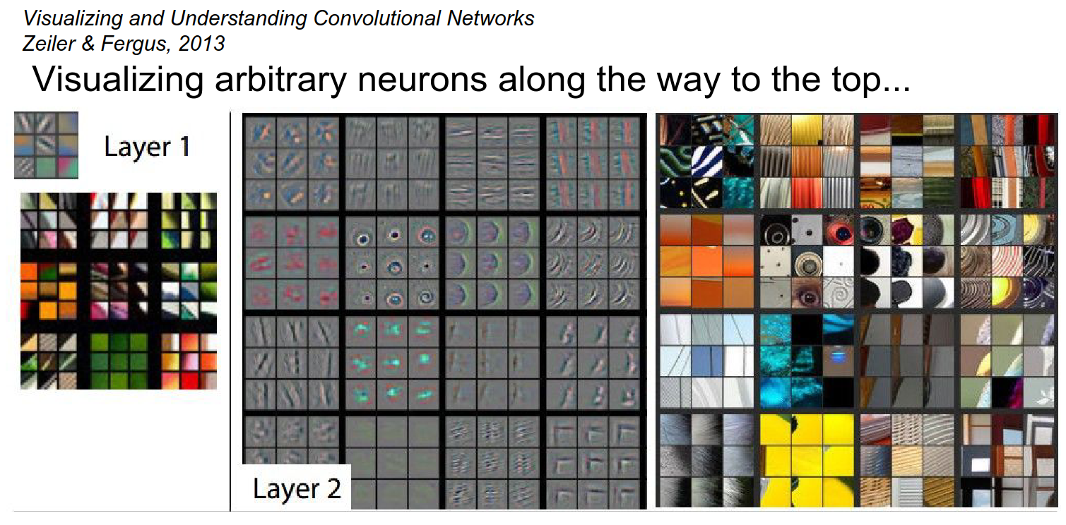
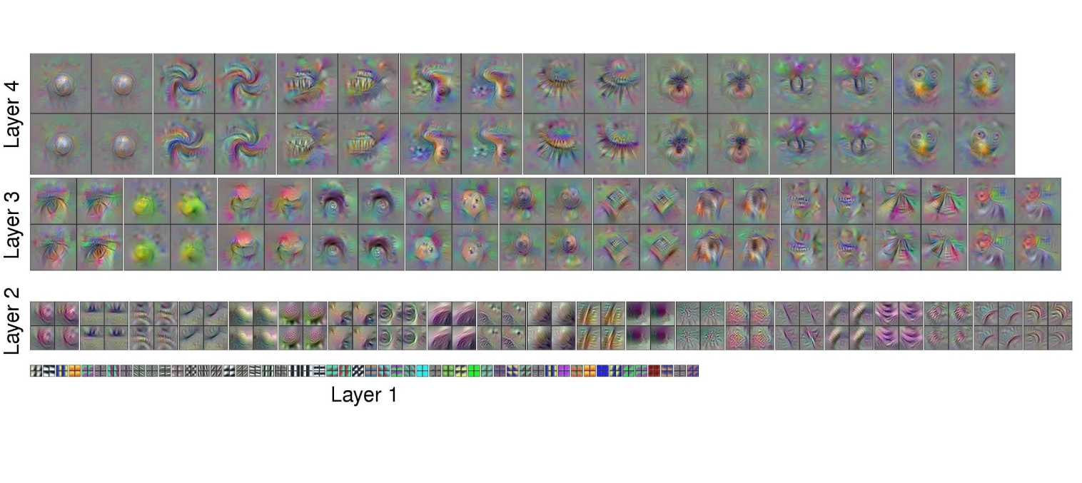
From Layer 3 onwards, you see shapes.
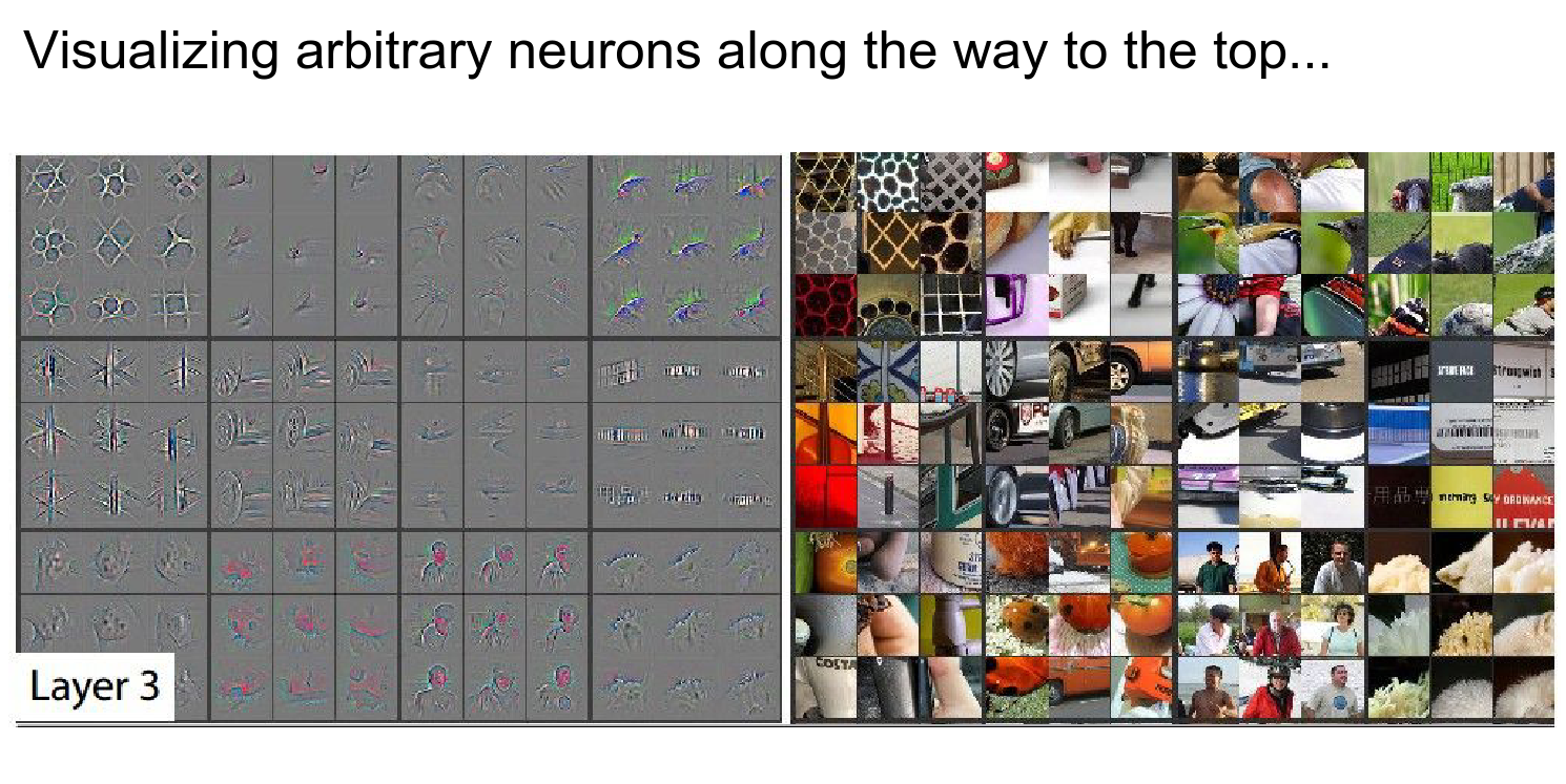
In the third row, third column, you see a human face as red. This means the gradient is telling you that if you made this person's face redder, it would have a locally positive effect on this neuron's activation.
Layer 4 starts to form objects.
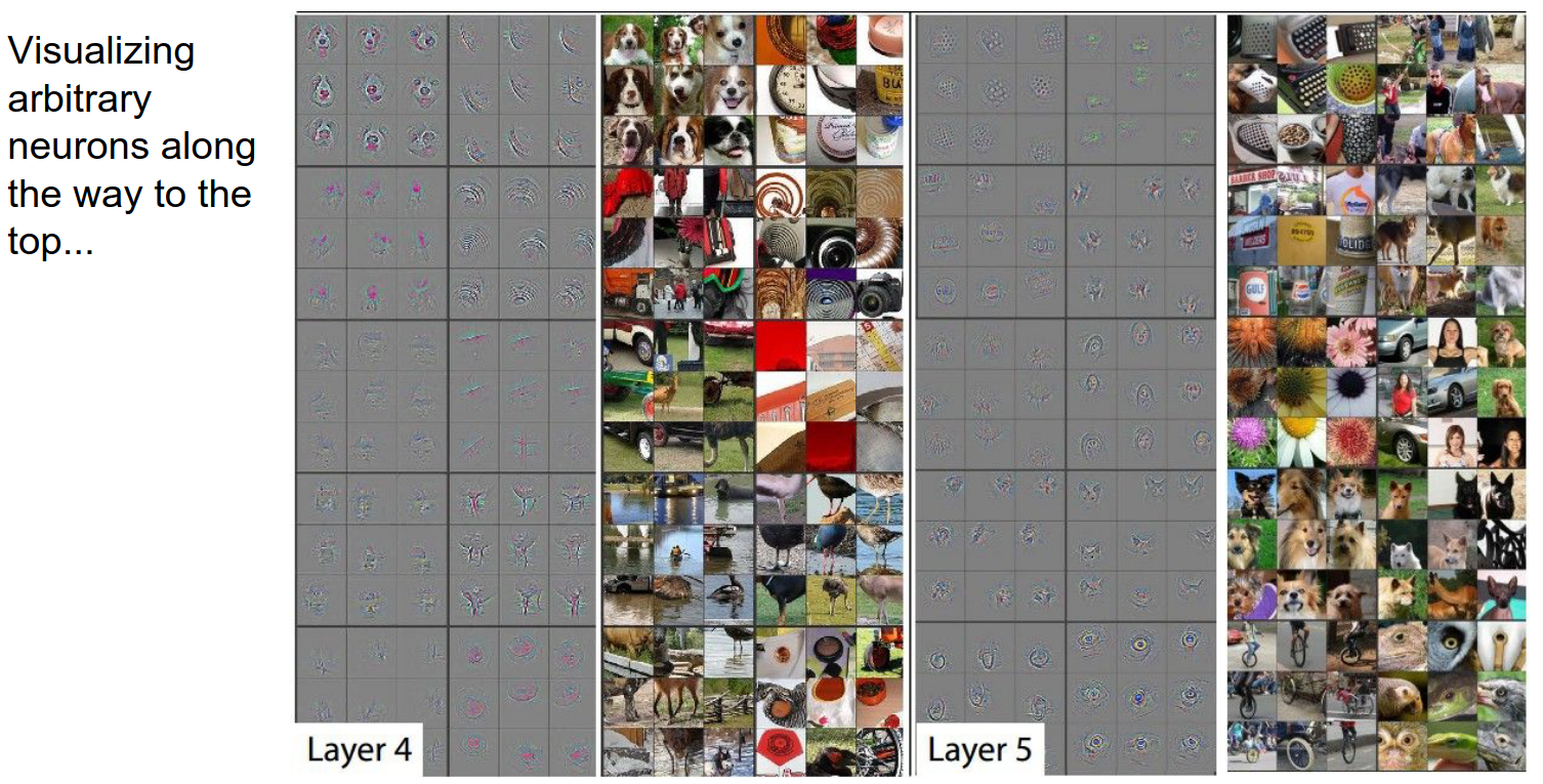
Andrej is not a big fan of the DeConv approach. You get pretty images, but that's about it.
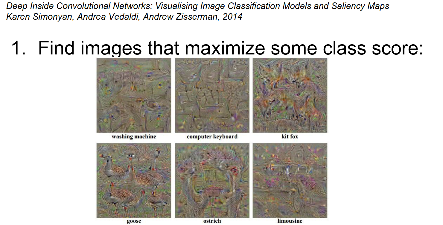
Optimization to Image
We will do a bit more work compared to the DeConv route.
We are going to try to optimize the image while keeping the Convolutional Neural Network fixed.
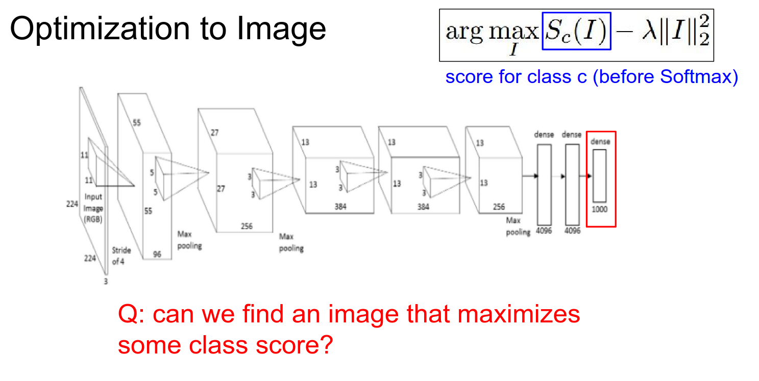
We are going to try to maximize an arbitrary score in the ConvNet.
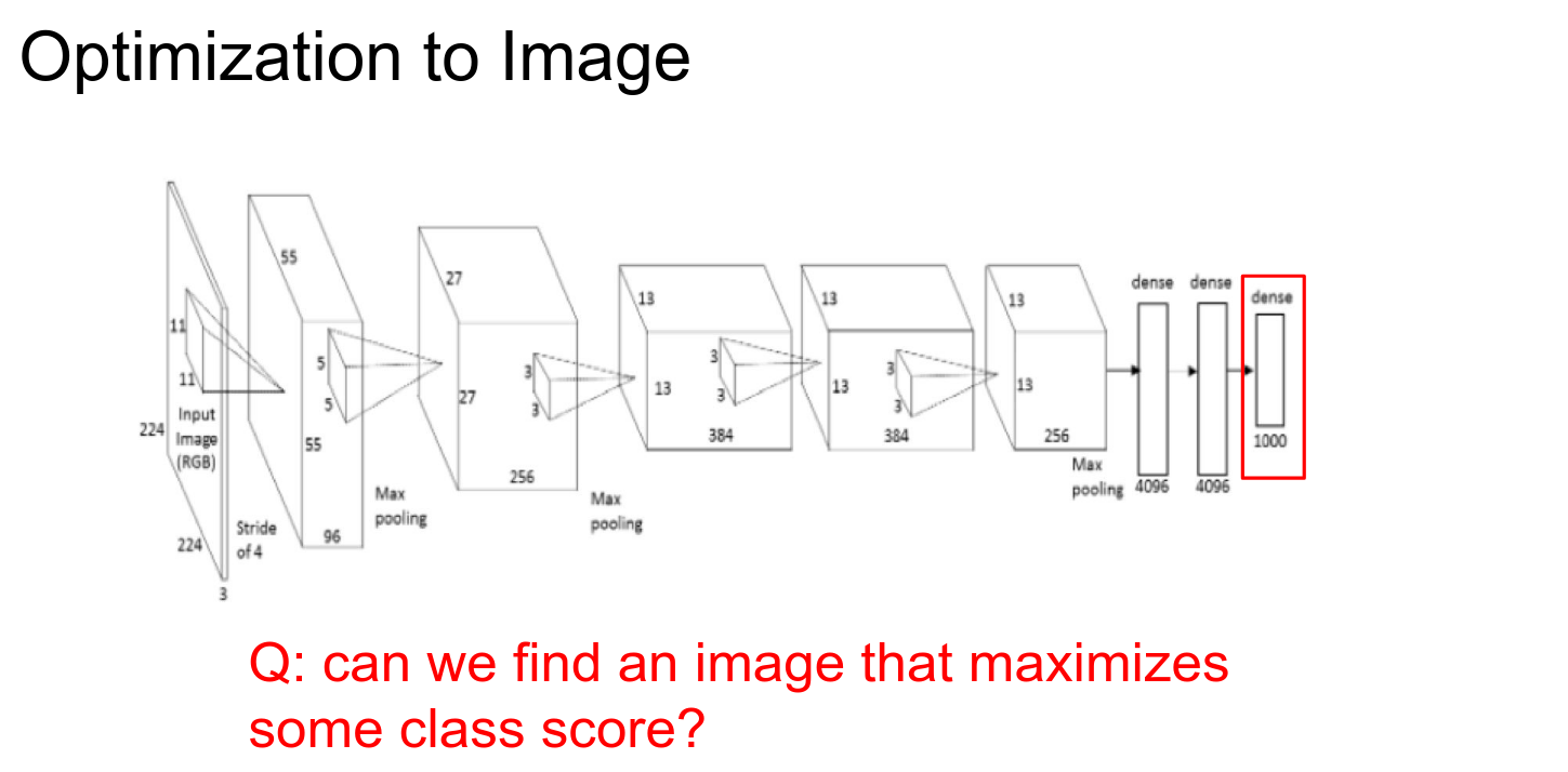
We are trying to find an image \(I\) such that your score is maximized, subject to some regularization on \(I\).
- L2 Regularization: Discourages parts of your input from being too large.
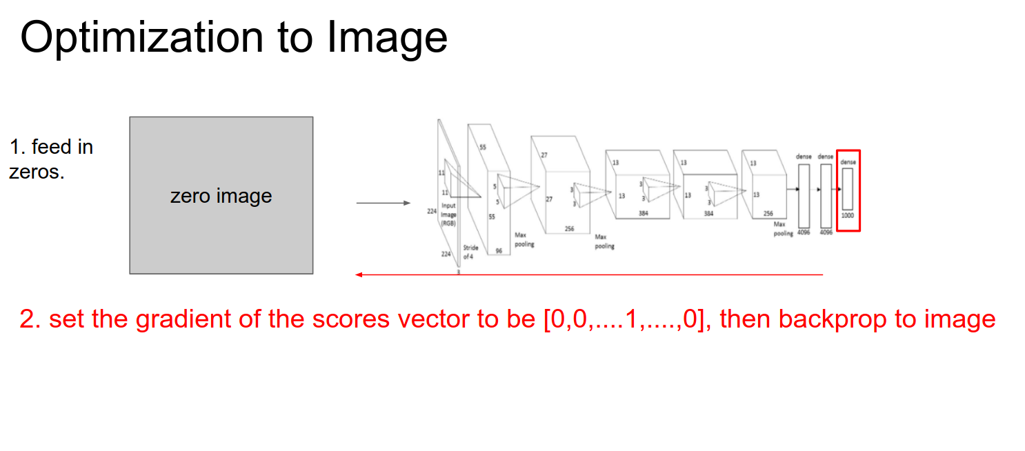
We start with a Zero Image. We feed it into a ConvNet.
We set the gradient at that point to be all 0s, except for a 1 at the neuron we are interested in.
This is just normal backpropagation.
We do a forward pass, a backward pass, and then updates.
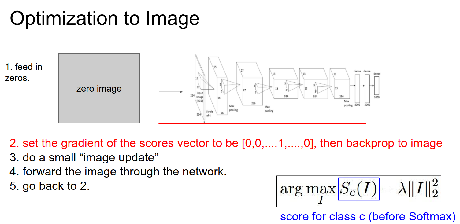
Iterate this over and over to optimize the image.
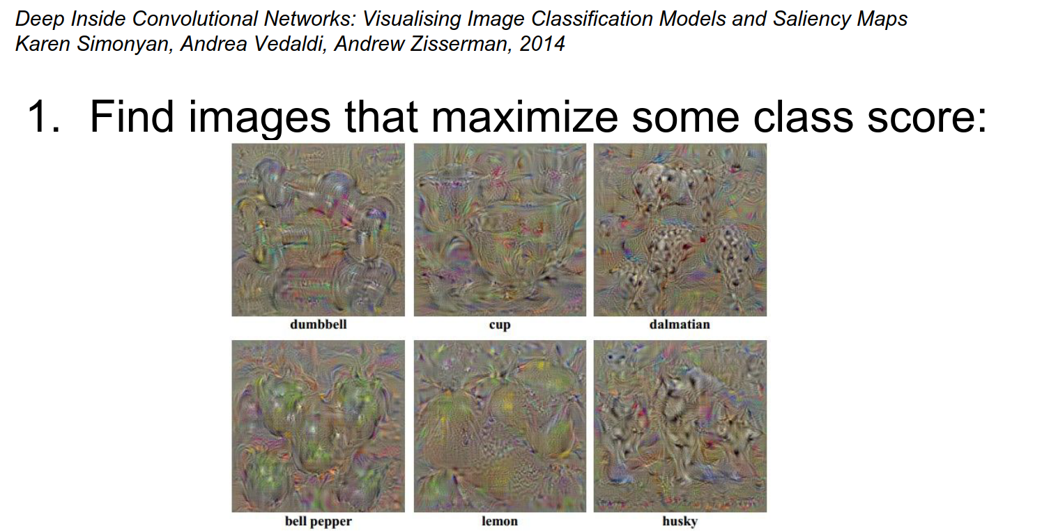
Geese Example 🥰
Another way of interpreting the gradient signal at the image is from the following paper:
Area of Influence
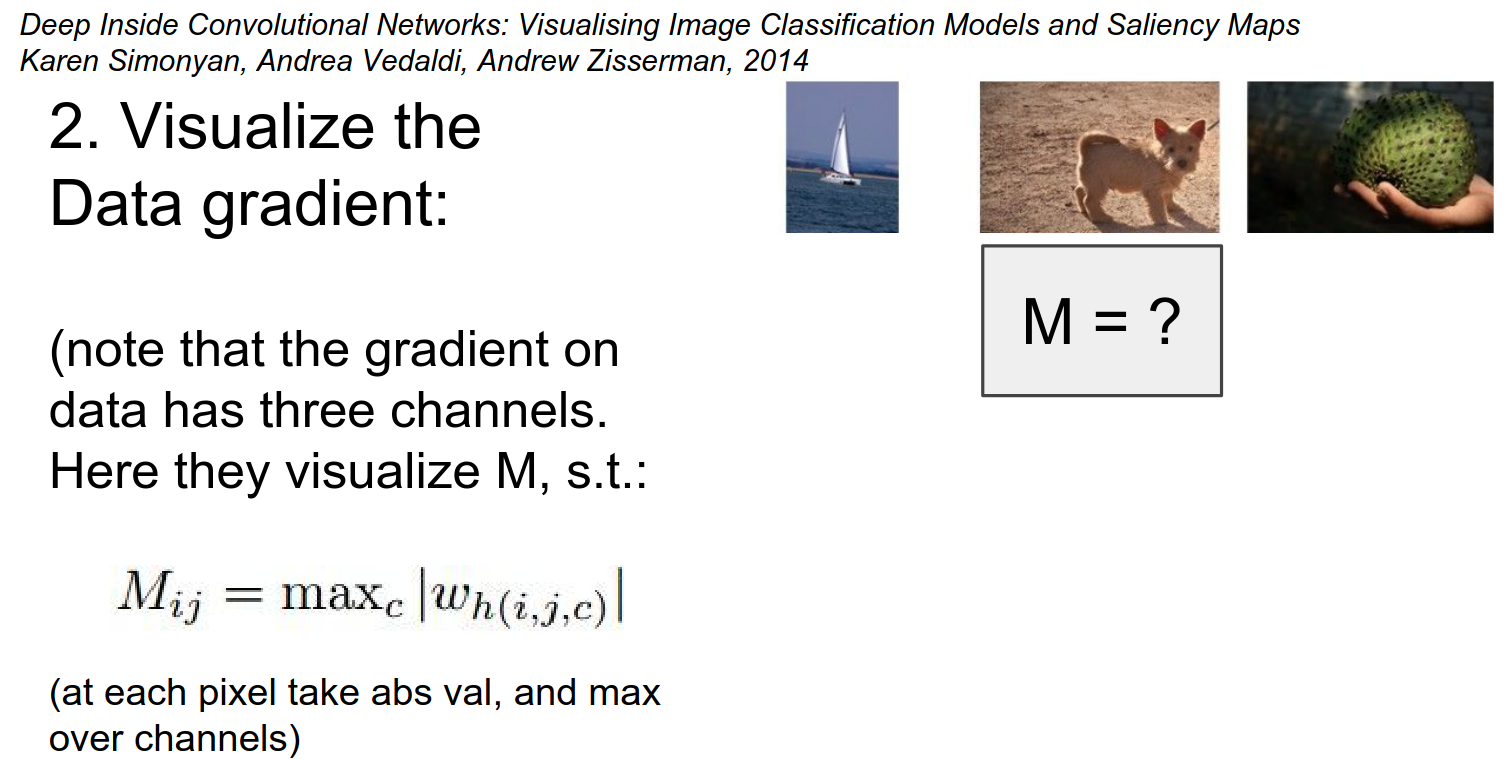
They forward the image (the dog), set the gradient to 1, and do backpropagation.
You arrive at your image gradient, and they squish it through channels with a \(max\) function.
What would you expect?
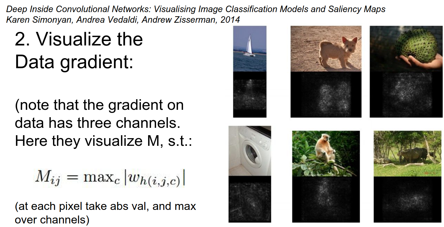
In the black parts of the image, if you wiggle a black pixel, the score for that image does not change at all. The ConvNet does not care about it.
So the gradient signal can be used (in a GrabCut segmentation) as a measure of the area of influence on the input image.
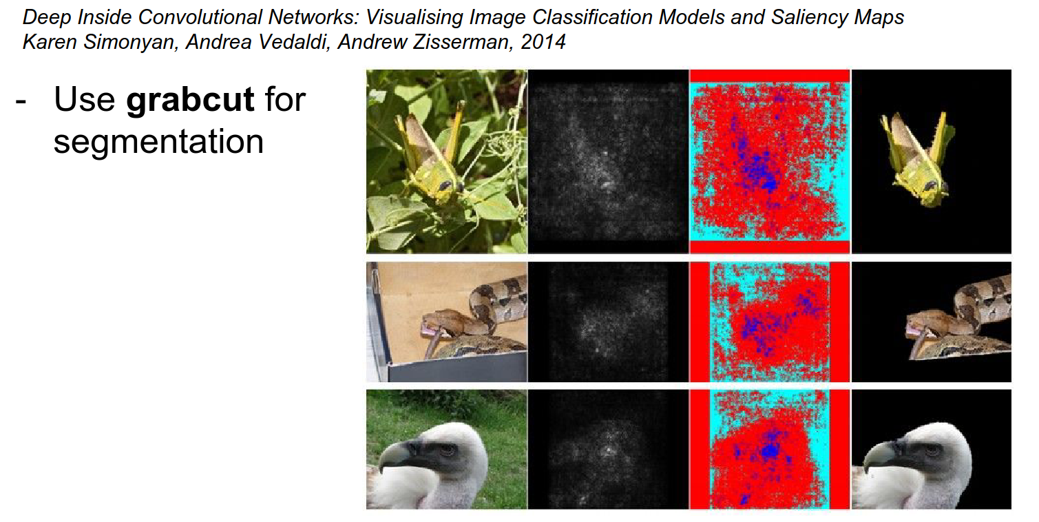
You can crop images just based on the gradient signal.
Seems suspicious -> Cherry-picked examples...
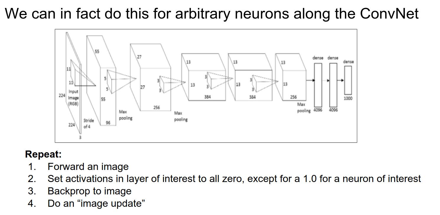
We were maximizing the full score and optimizing the image. We can do this for any arbitrary neuron.
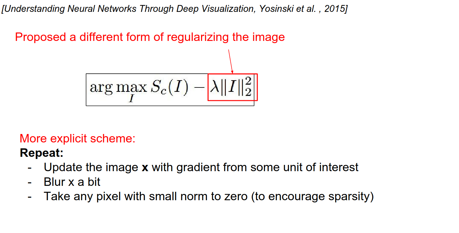
We have been using L2 penalty so far. Is there a better way?
- Ignore the penalty.
- Do forward and backward passes.
- Blur the image a bit (this prevents the image from accumulating high frequencies).
- This blurring will help you get cleaner visualizations for classes.
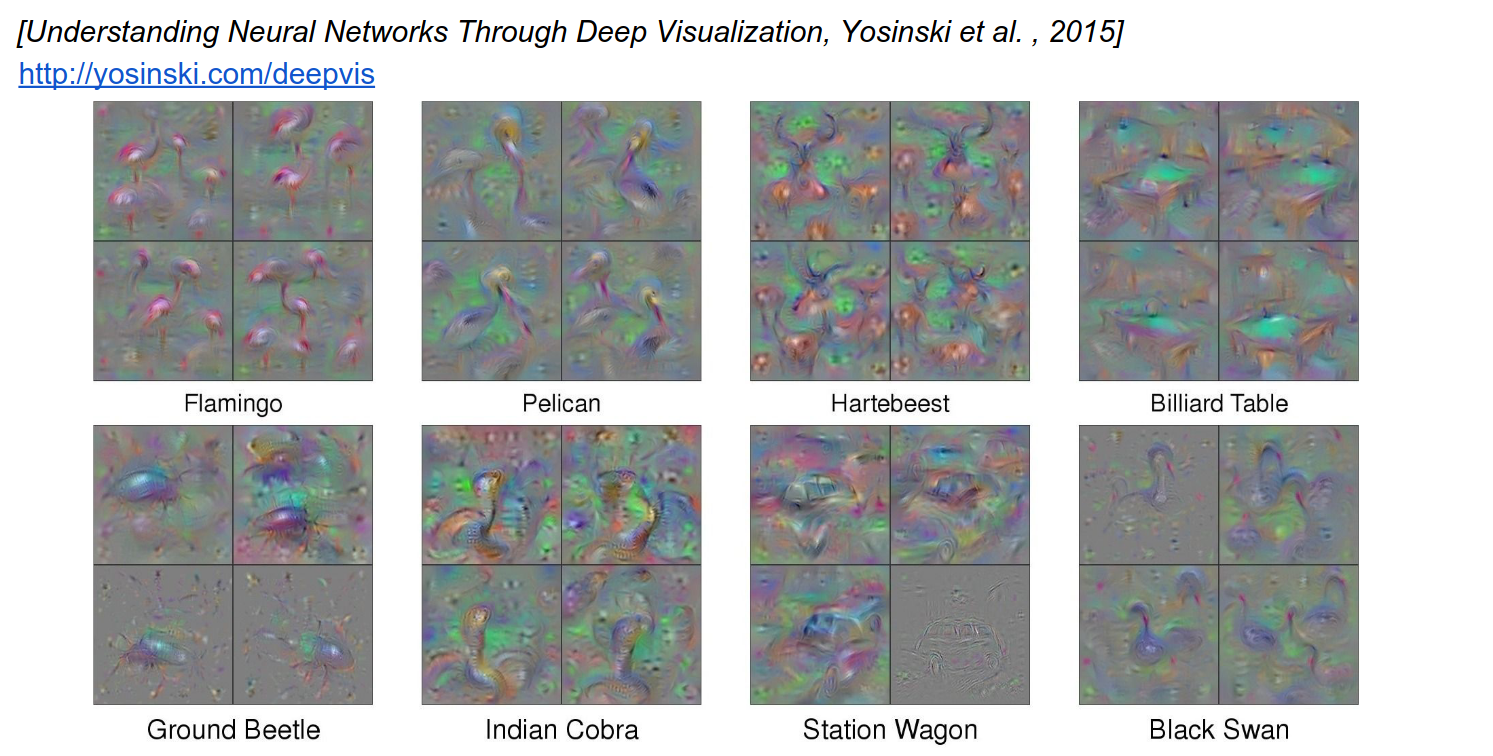
This looks a bit better. 4 different results with 4 different initializations.
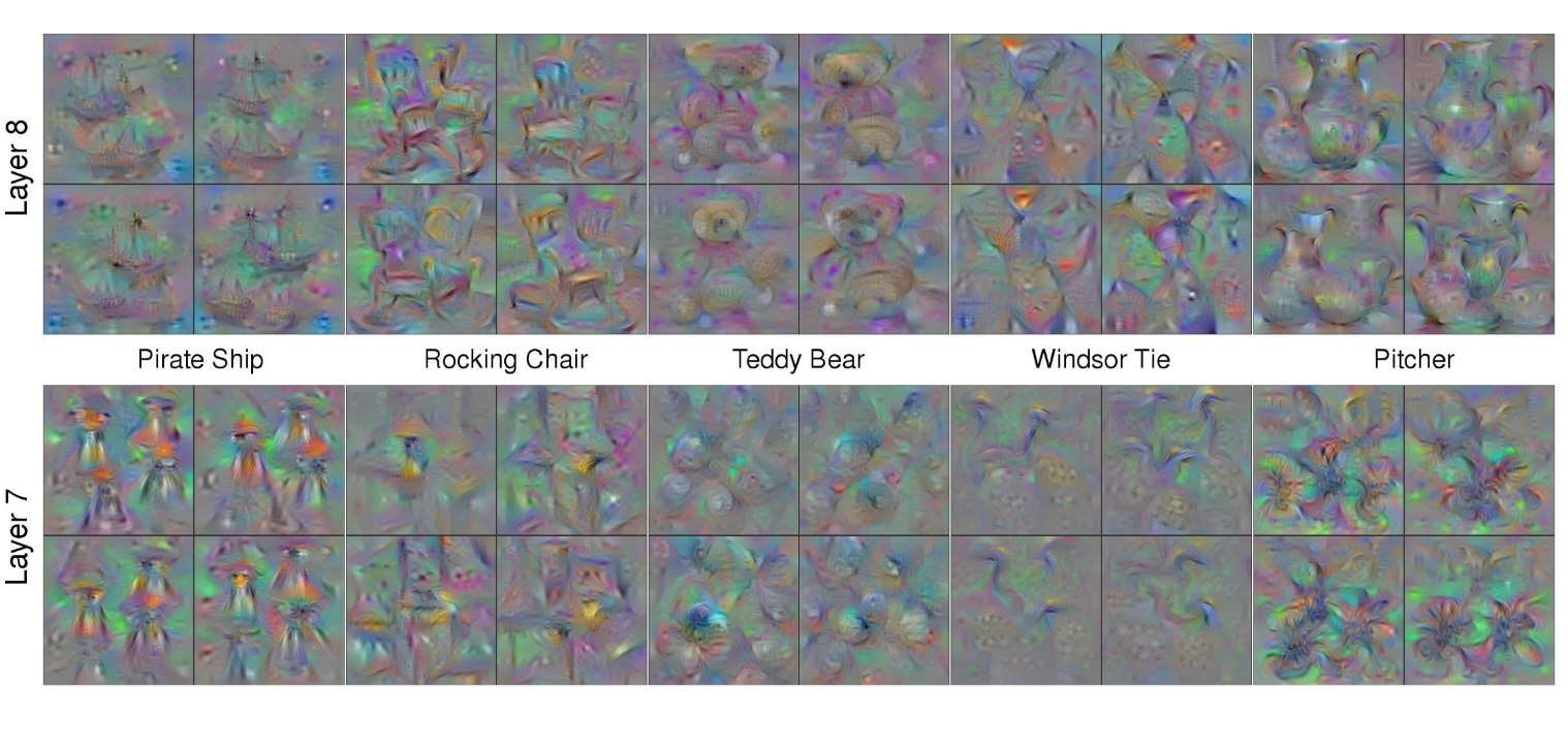
You can go down layers to see.
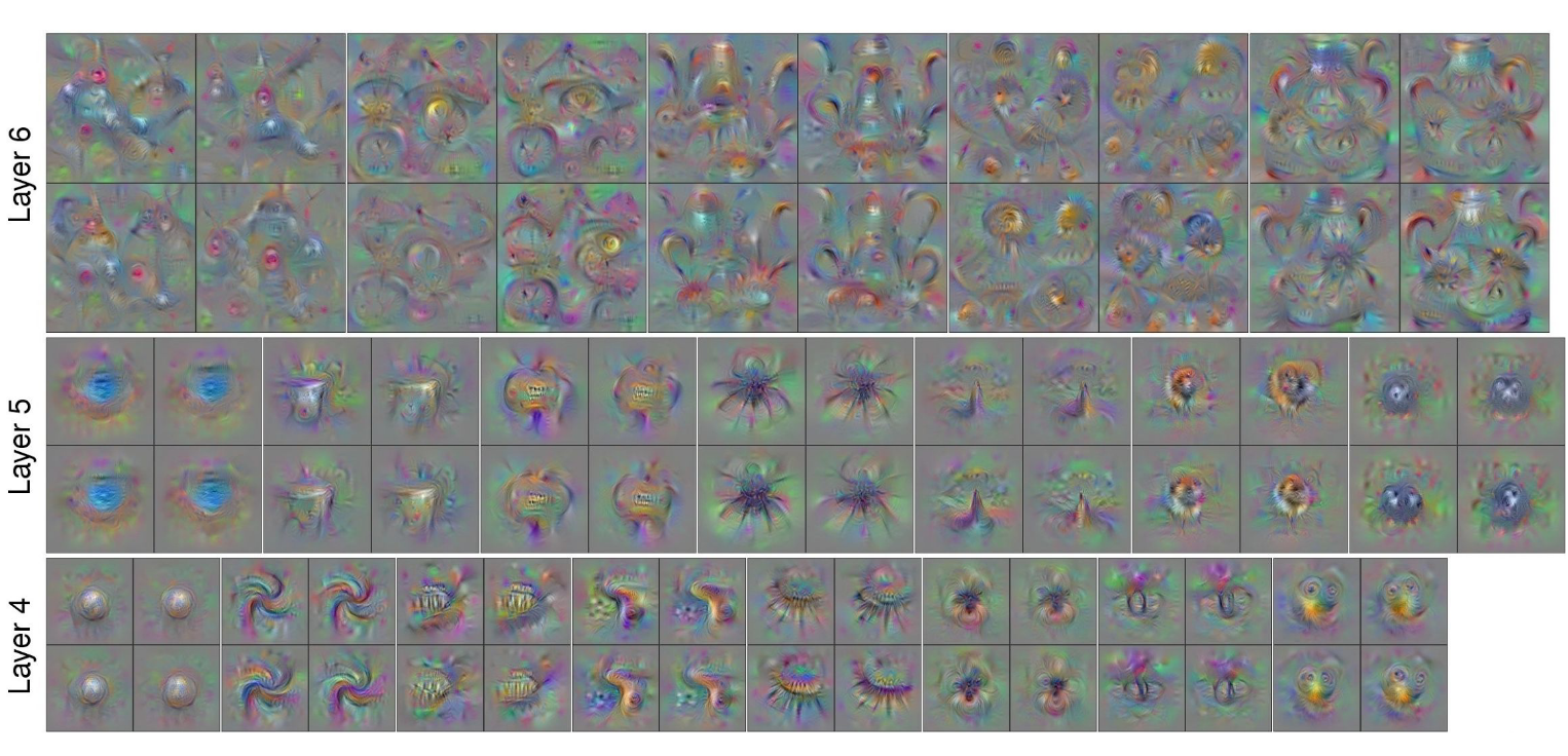
In Layer 5, there is some part of an ocean.
These just come out of the optimization. This is what these neurons really like to see.
Effective Receptive Field
In the first layer of VGG, it is just \(3x3\). As you go down, the effective receptive field gets bigger. So you see neurons that are functions of the entire image.
Information Content
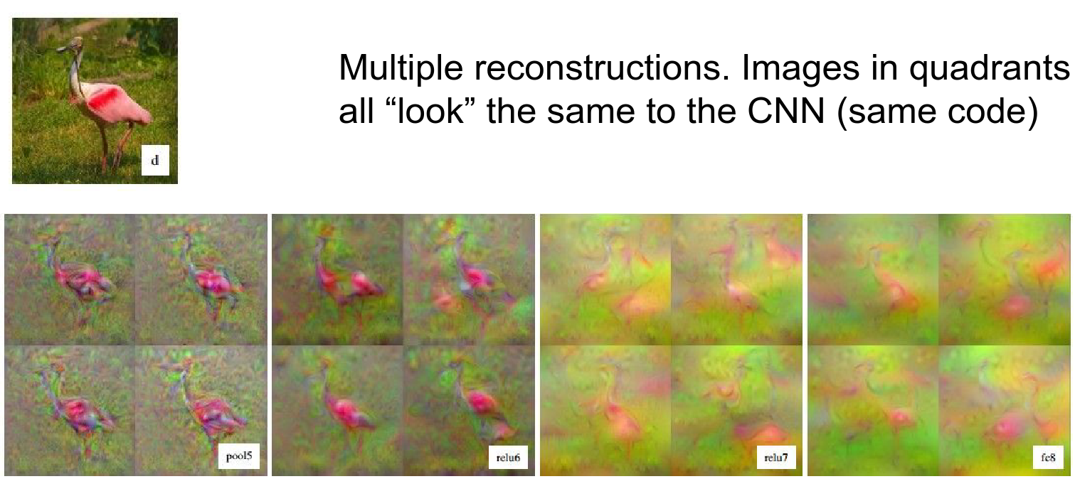
Can you invert the image with just the code?
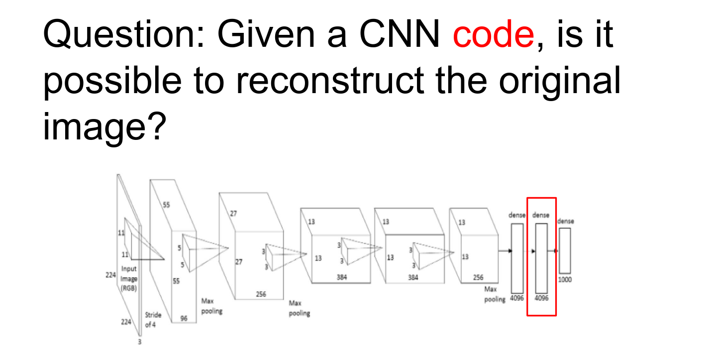
- We are given a particular feature.
- We want to find an image that best matches that code.
Instead of maximizing any arbitrary feature, we just want to have a specific feature and exactly match it in every single dimension.
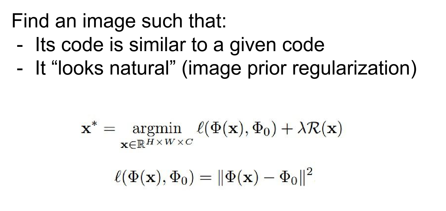
When you run the optimization, you will get something like this.
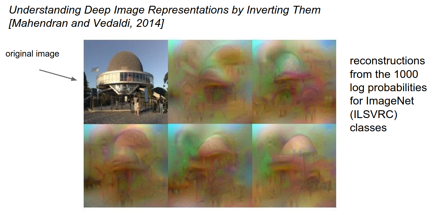
You can do reconstruction at any place in the ConvNet. The example below is even better than our first one.
The bird location is pretty accurate, so this is proof that the code is rich in information.
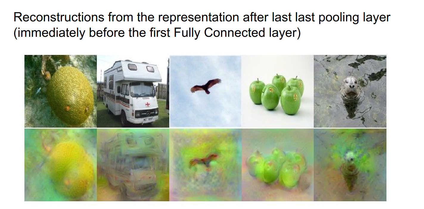
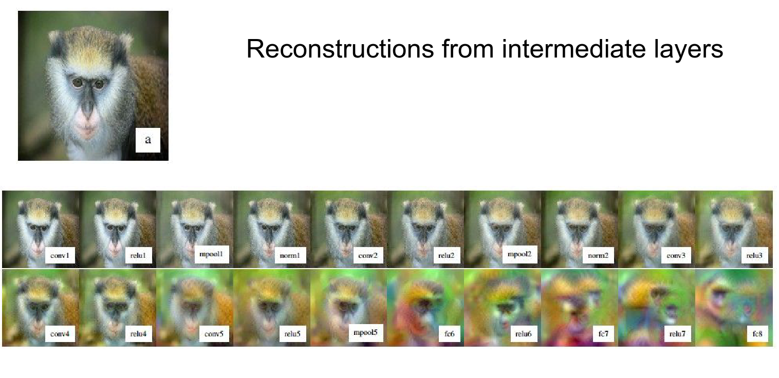
You can also look at a single image and see how much information is thrown away as you move forward.
You can compare reconstruction at different layers. When you are very close to the image, you can do a very good job of reconstruction.
A flamingo example:
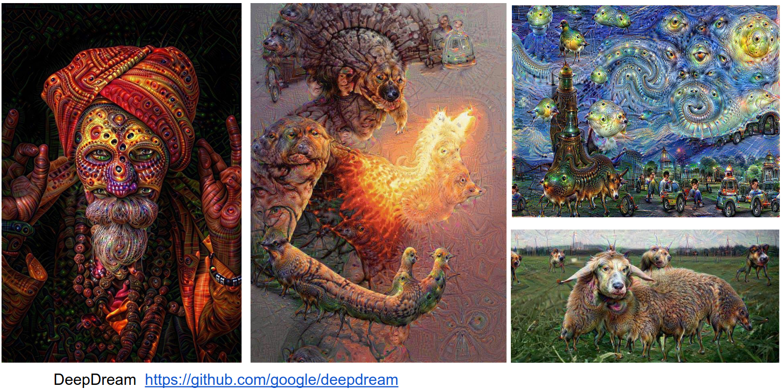
You can get really funky images as you try to optimize the image. It's 100 lines of code in a Python notebook.
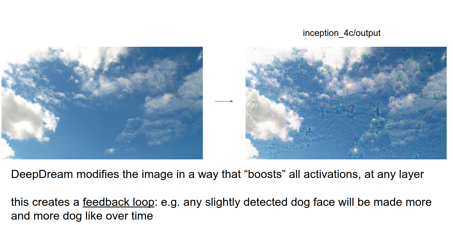
This is based on an Inception network. We choose the layer we want to dream at.
make_step will be called repeatedly.
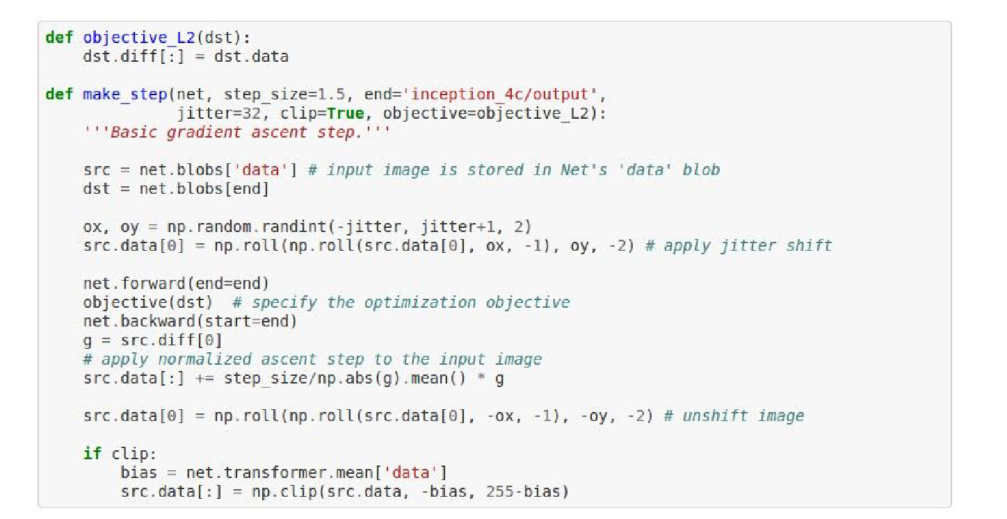
We forward pass the network, call the objective on the layer we want to dream at, and then do a backward pass.
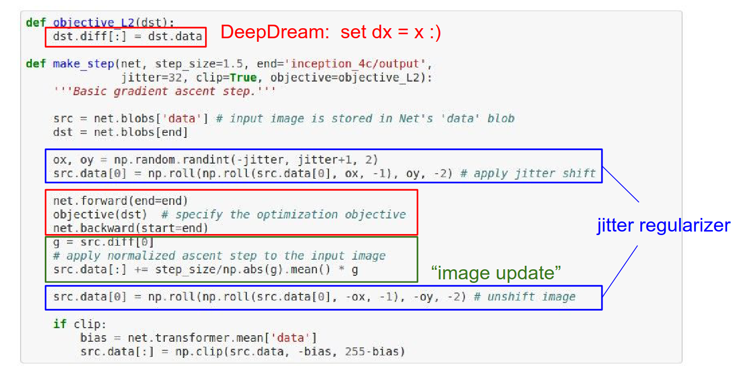
You have a ConvNet. You pass the image through to some layer where you want to dream. The gradients at that point become exactly identical to the activations at that point. Then you backpropagate to the image.
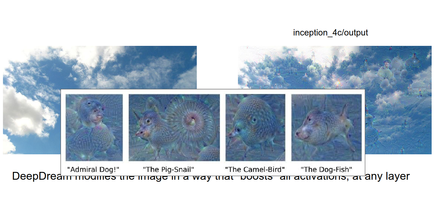
There are so many features that really care about dogs because there are so many of them in the training data for ImageNet. A large portion of ConvNet features really like dogs.
We want to boost what we know. If a cloud resembles a dog, the image will be refined to be more dog-like.
Funky things.
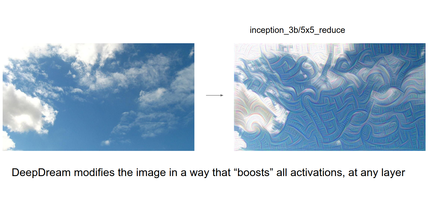
If you DeepDream lower, the features are more like edges and shapes.
Funny videos.
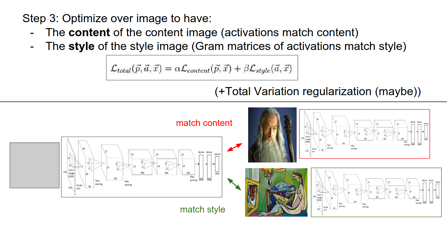
Neural Style
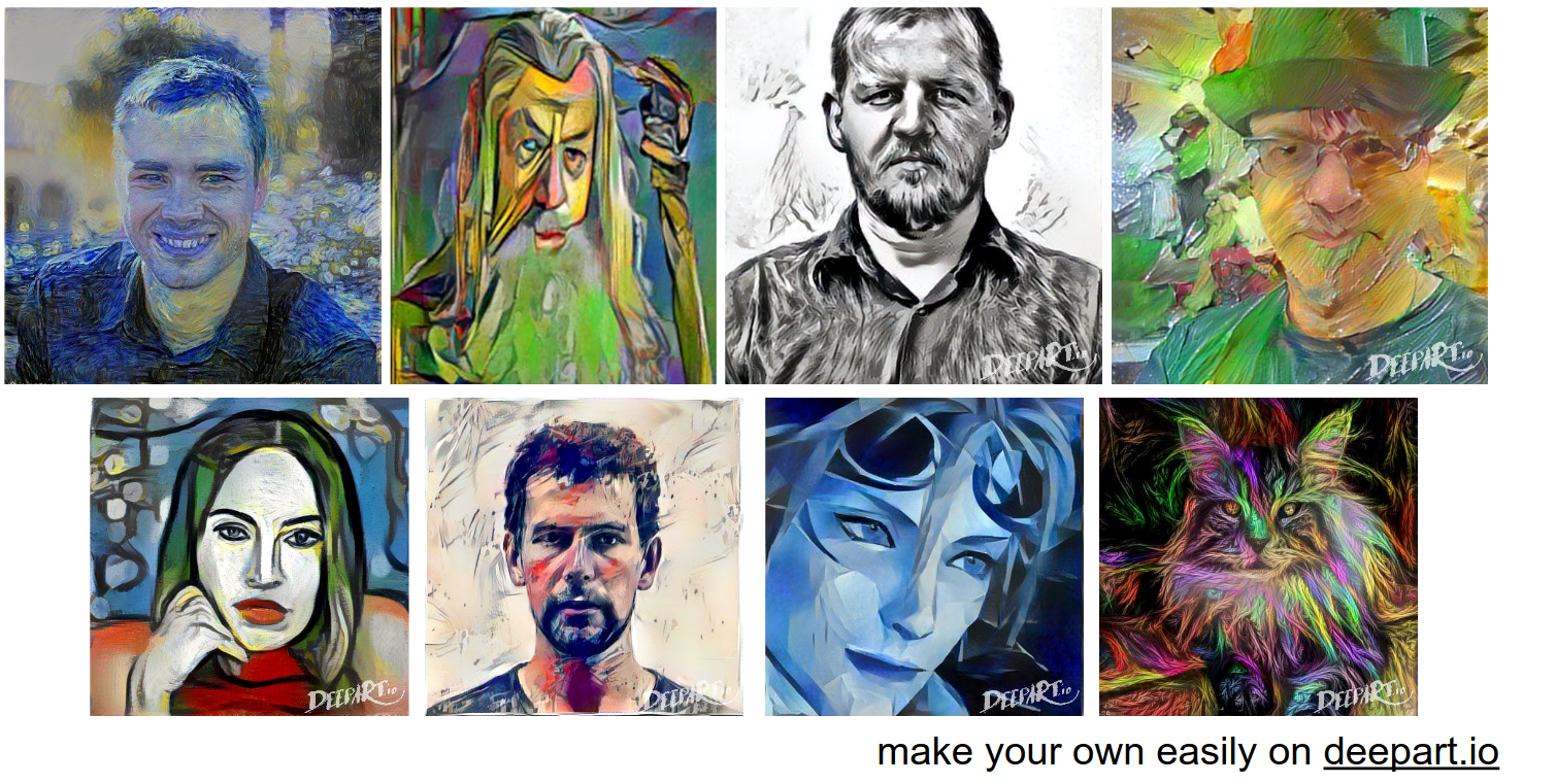
You can take a picture and render it in a different style.
This is achieved by Optimization on the raw image with ConvNets.
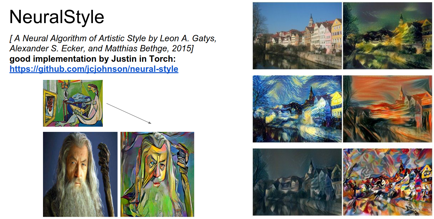
Examples:
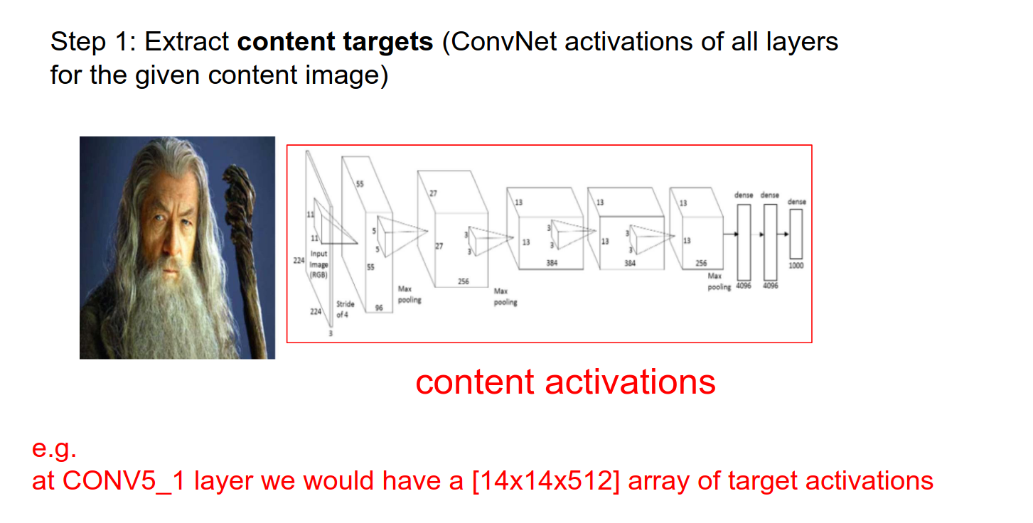
We have a content image and a style image.
We pass the content image into the ConvNet. We hold the activations as they represent the content.
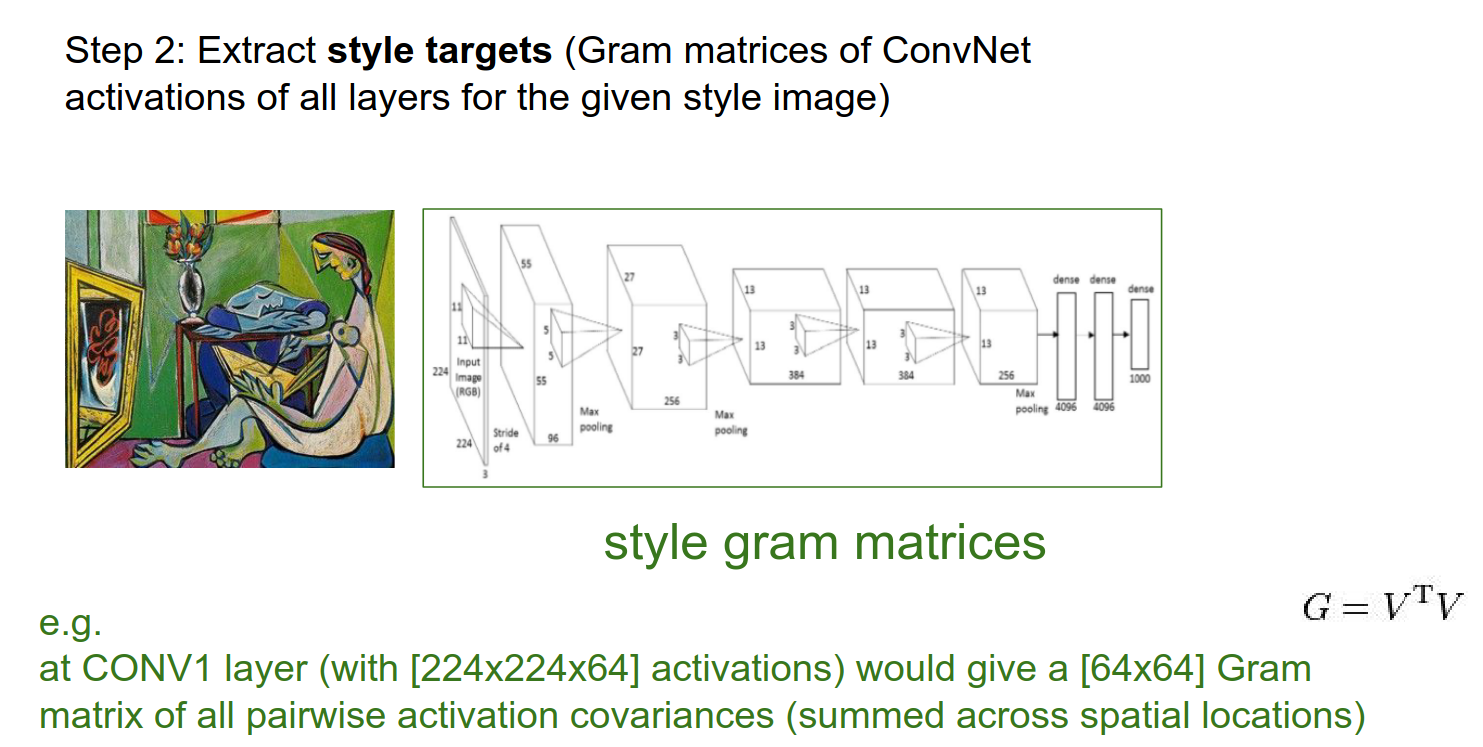
We take the style image and pass it through the ConvNet.
Instead of keeping track of the raw activations, the paper authors found that the style was not in the raw activations but in their pairwise statistics.
We got a \(224x224x64\) activation at the Conv1 Layer. We want some fibers from it. \(64x64\) (Gram matrices) is what we want.
Feature Correlations
We will do this on every Conv layer.
- We want to match the content (all the actual activations from content) and style (the Gram matrices).
- These 2 objectives are fighting it out.
- In practice, we run content in Layer 5 (a single layer) and use many more layers for style.
This is best optimized with L-BFGS. We do not have a huge dataset, everything fits in memory, so second-order methods (instead of Adam, AdaGrad) work really well here.
Adversarial Examples
We saw all the optimizations on the image.
You can make a school bus, or anything, into an ostrich.
We get the gradient on that image for the Ostrich class.
We forward the image. We set all gradients to 0 except for the class we want (ostrich). We do a backward pass, and we get a gradient of what to change in the image to make it more like an Ostrich.
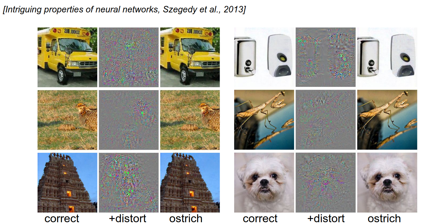
The distortion you need is really small. You can turn anything into anything.
You can start from random noise.
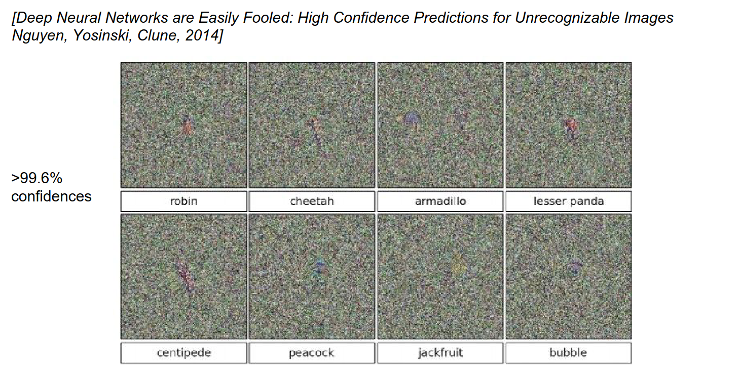
You can use weird geometric shapes.
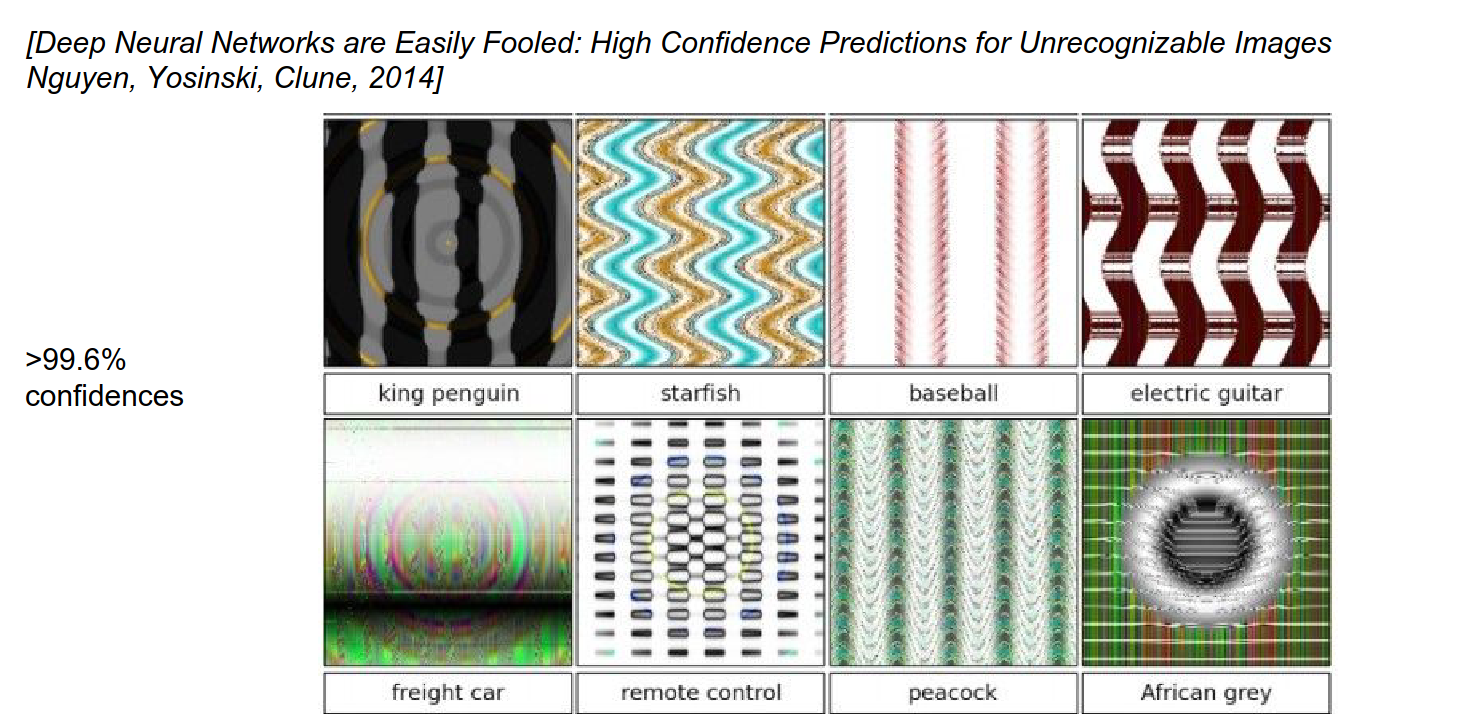
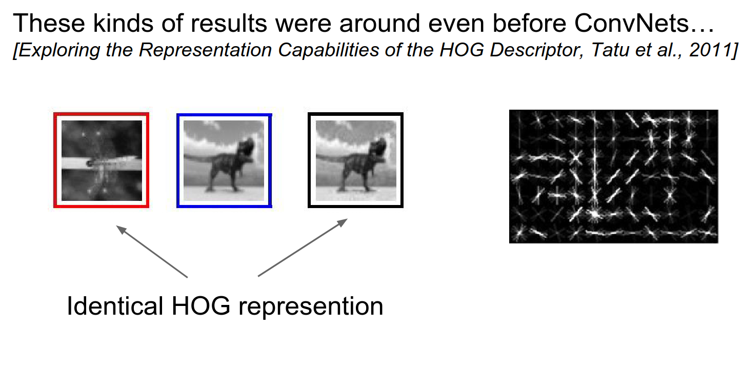
This is not really new; this happened before.
HOG representation is identical, but the images are so different from each other.
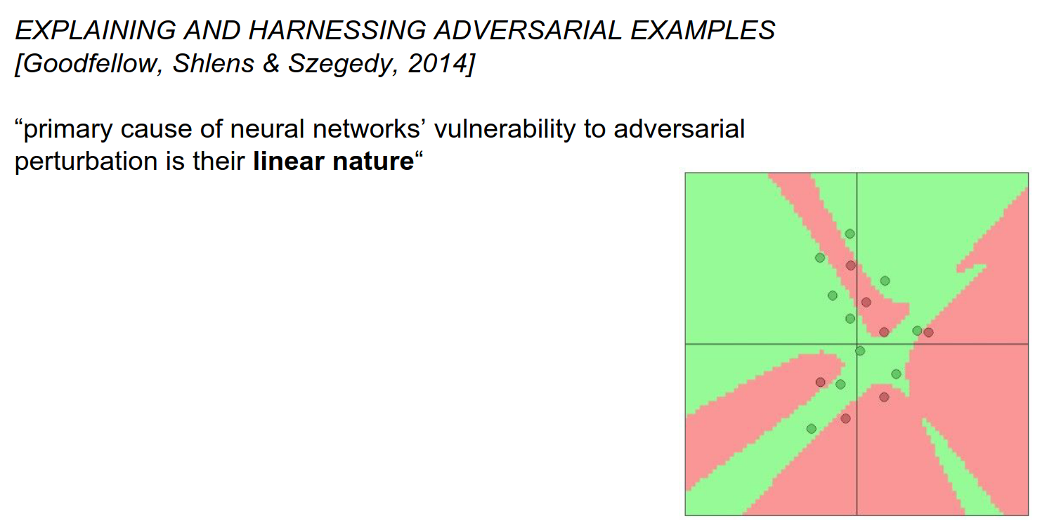
Manifold Hypothesis
Images are super high-dimensional objects (150,000-dimensional space).
Real images that we train on have a special statistical structure and are constrained to tiny manifolds in that space.
We train ConvNets on these. These ConvNets work really well on that tiny manifold, where the statistics of images are actually image-like.
We are putting these linear functions on top of it. We only know a little part; there are a lot of shadows.
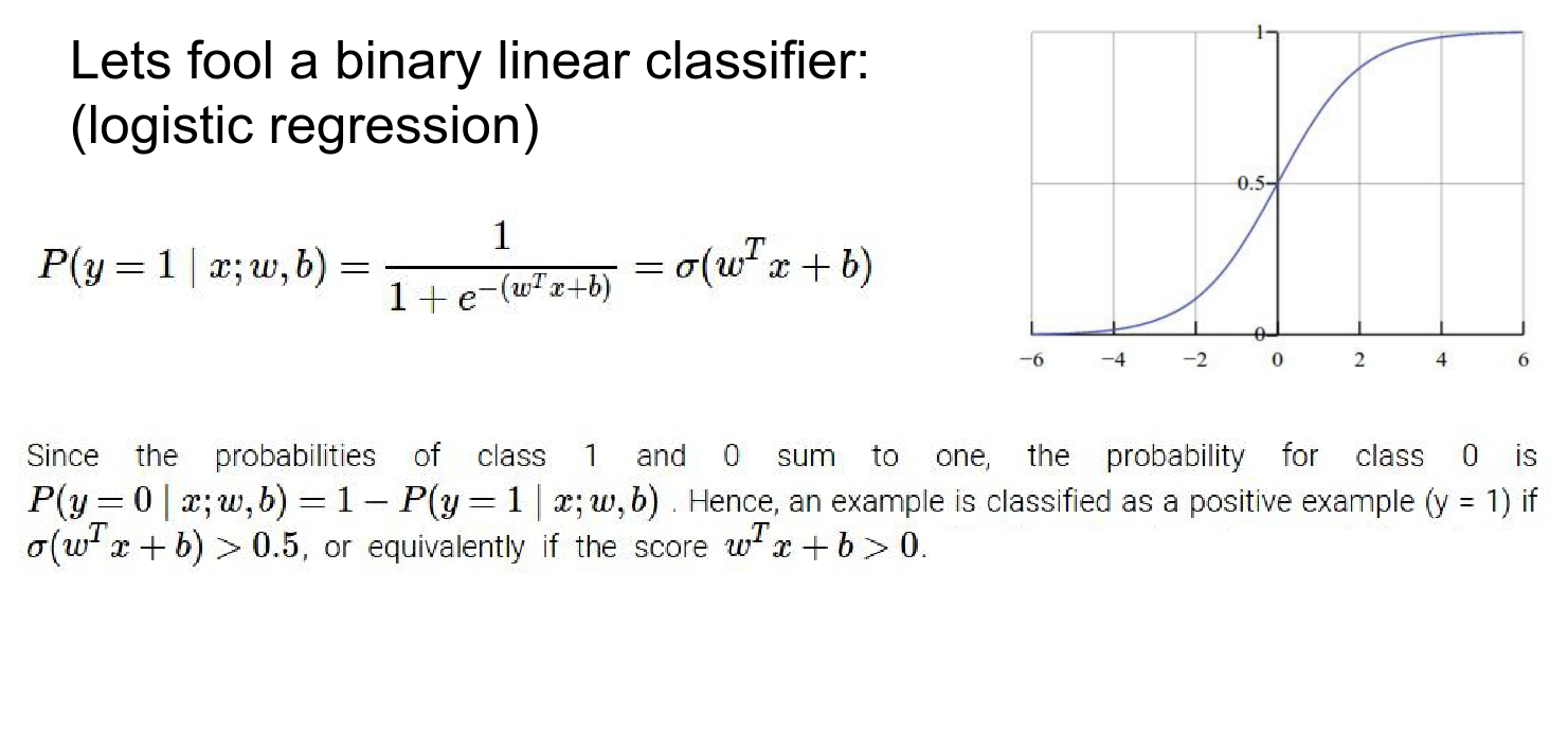
Let's just work with logistic regression.
\(x\) is 10-dimensional. \(w\) is a multi-dimensional vector and \(b\) is bias.
We put that through a sigmoid. We interpret the output of that sigmoid as the probability that the input \(x\) is of class 1.
We compute the score with this classifier. The input is class \(1\) if the score is greater than 0 (or equivalently, if the sigmoid output is greater than \(0.5\)).
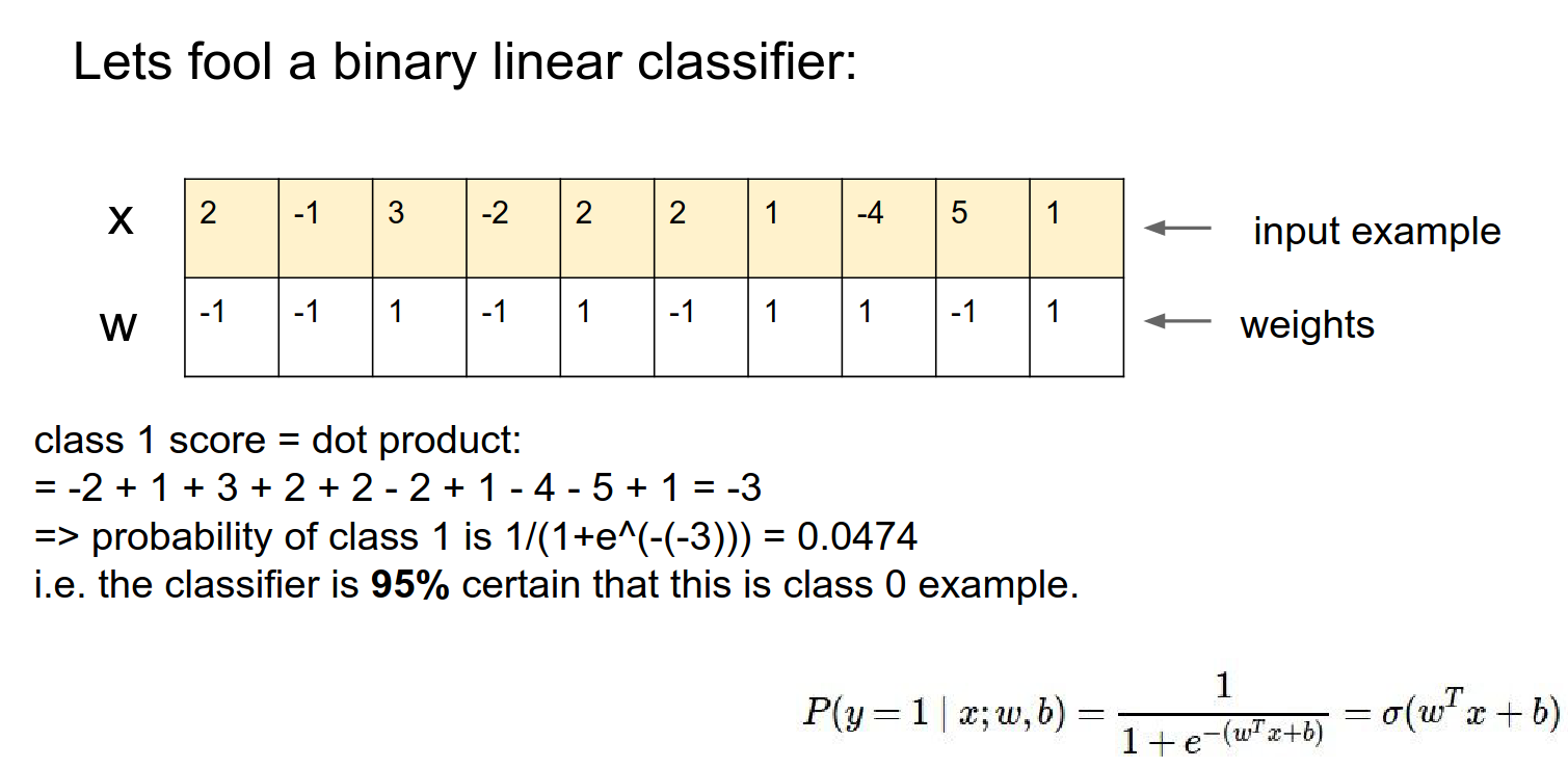
No bias example:
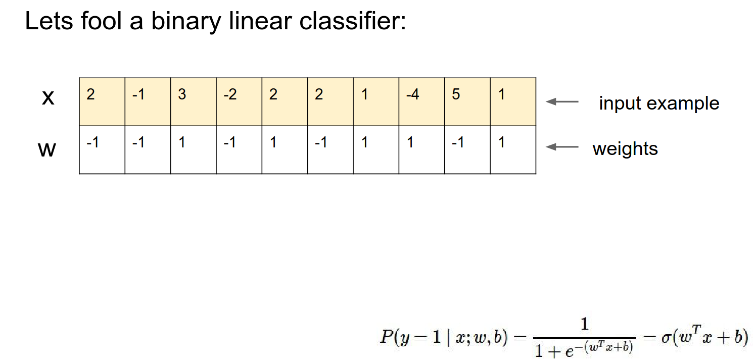
Just the dot product of the vectors. With this setting of weights, this classifier thinks it's 95% class 0.
Adversarial Perturbations
We want to slightly modify \(x\) and confuse the classifier.
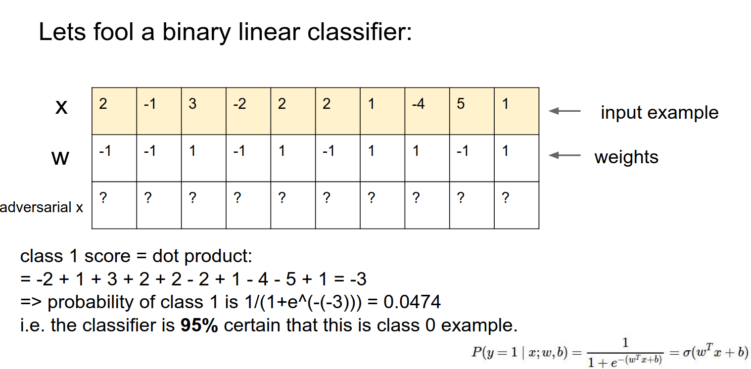
We want to make really tiny changes. We can do this in every single column.
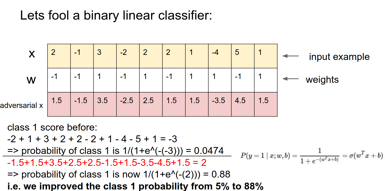
All the changes add up together.
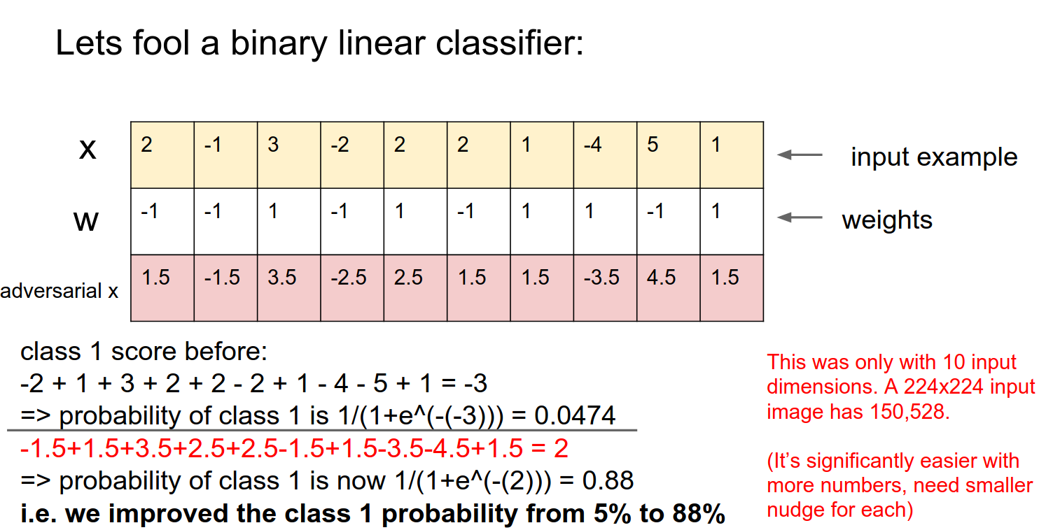
We blew out the probability. This was just a small number of inputs.
In images -> We can nudge 150,528 pixels in a really small way, and we can get any class we want.
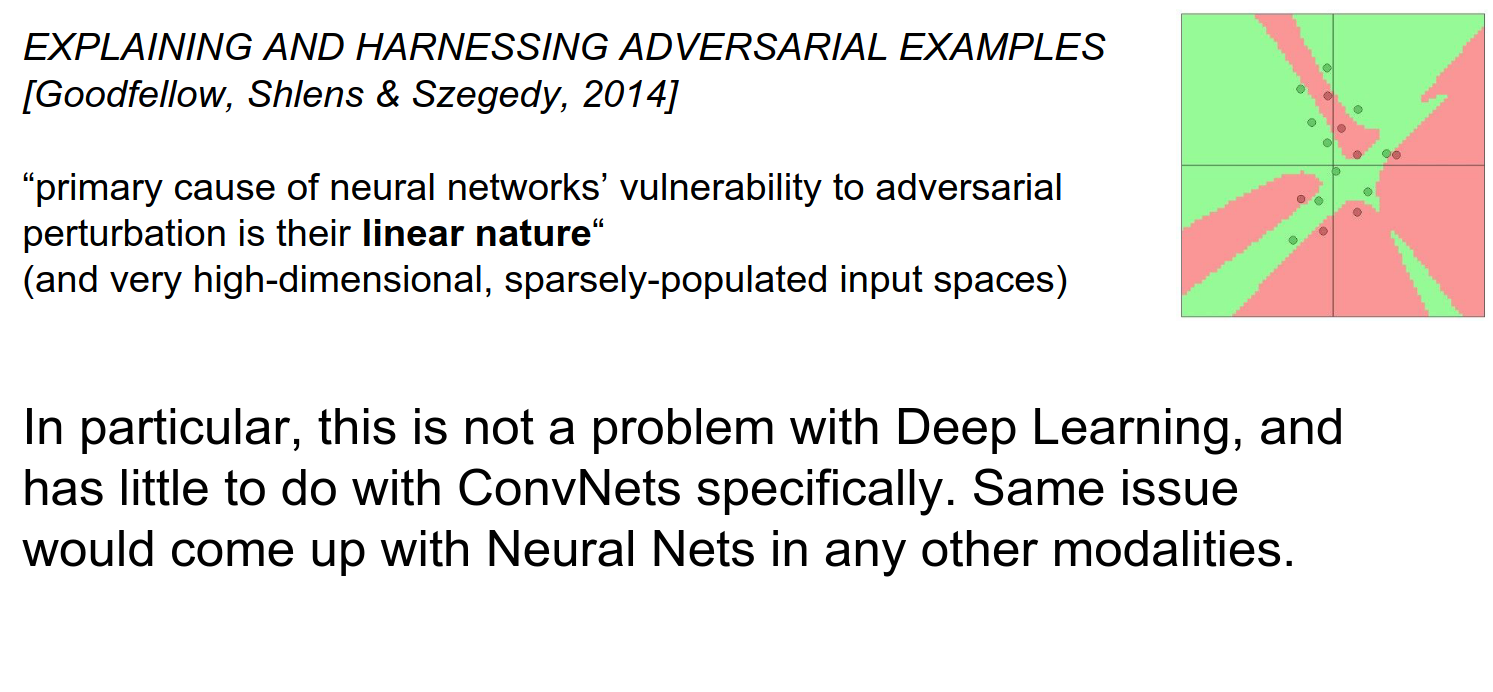
We can do this in linear classifiers (it has nothing to do with deep learning or ConvNets).
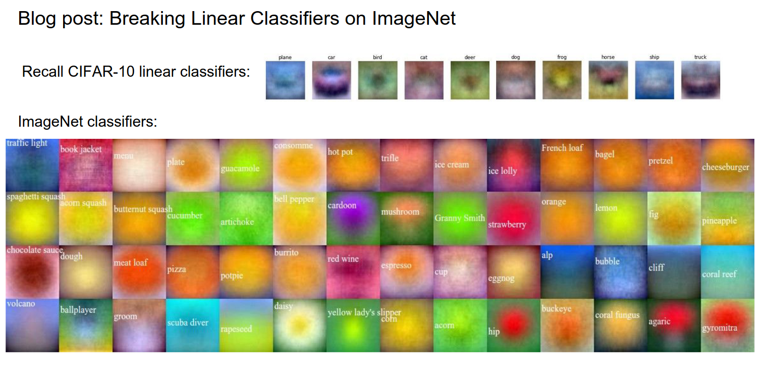
We can make templates for all datasets.
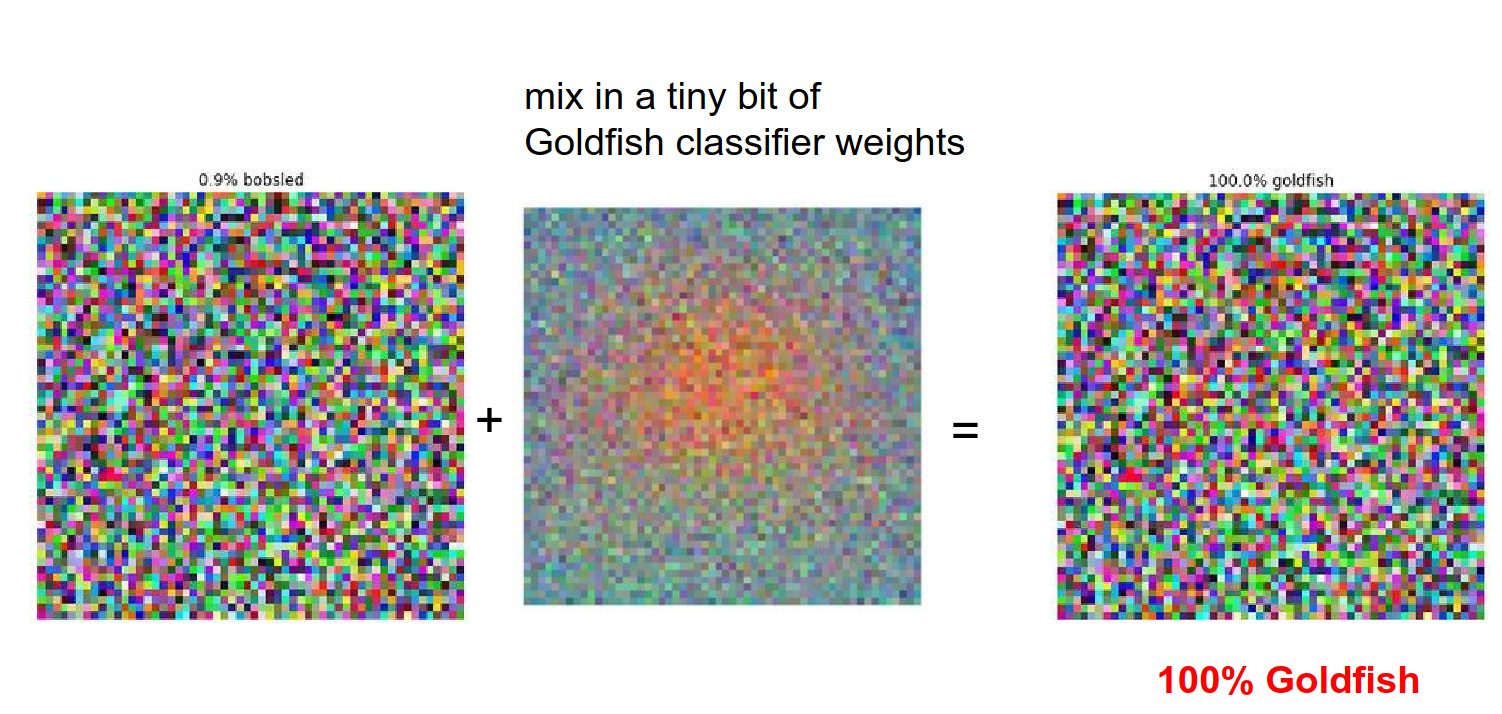
We can mix a bit of Goldfish weights -> 100% goldfish.
We can do this with original images altered too.
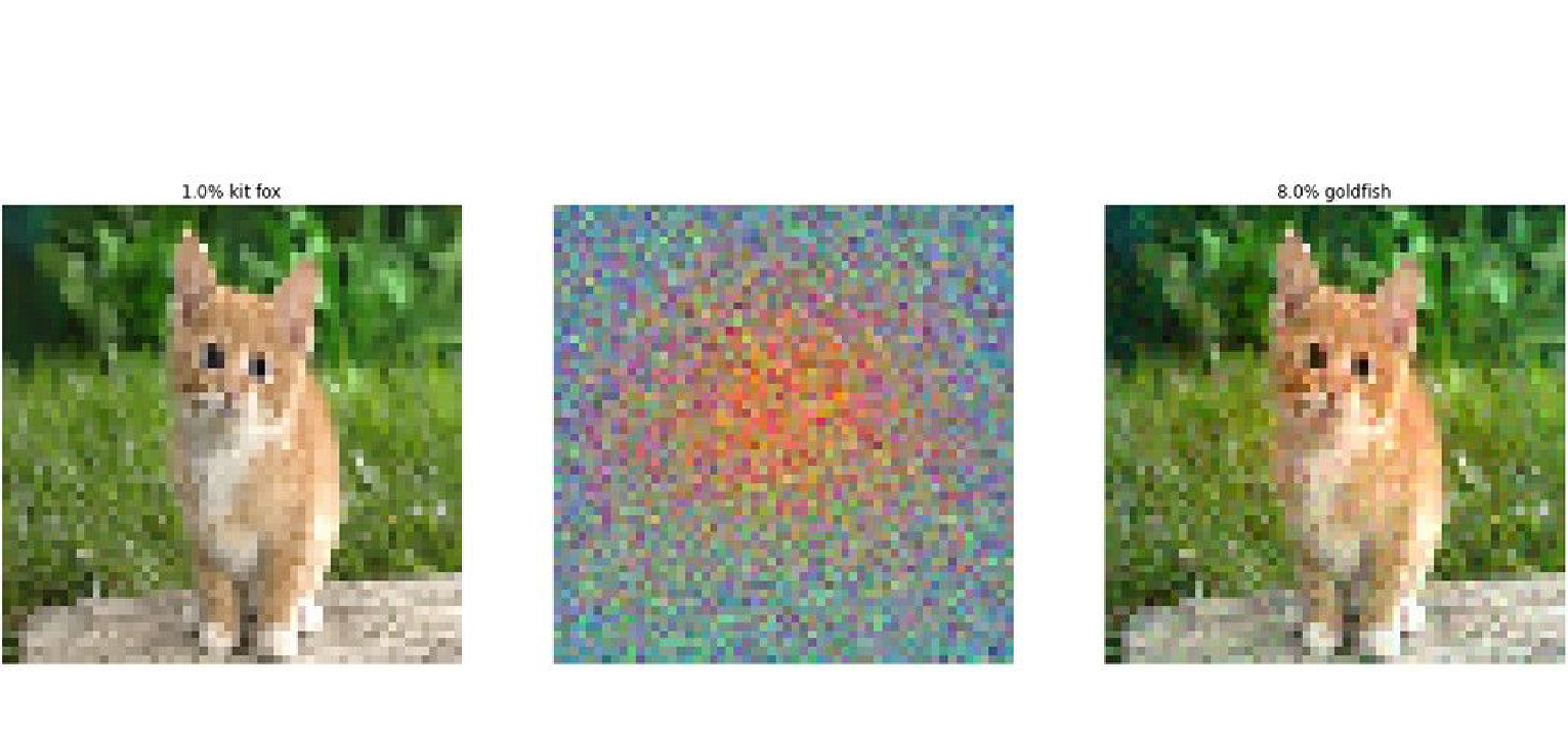
We can make a goldfish into a daisy.
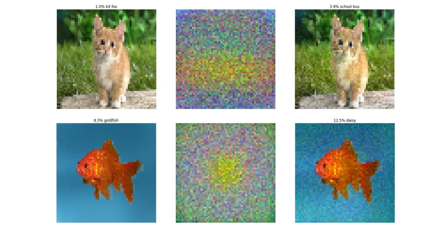
This has nothing to do with ConvNets or Deep Learning.
We can do this in any other modality, like speech recognition too.
To prevent this, you can train the ConvNet with parts of the image or augmentations to make it a little stronger.
You can try to train the ConvNet with training data and adversarial examples (as negative scores), but you can always find new adversarial examples.
You can change the classifier, and this kinda works, but now your classifiers do not really work as they used to.
Implications
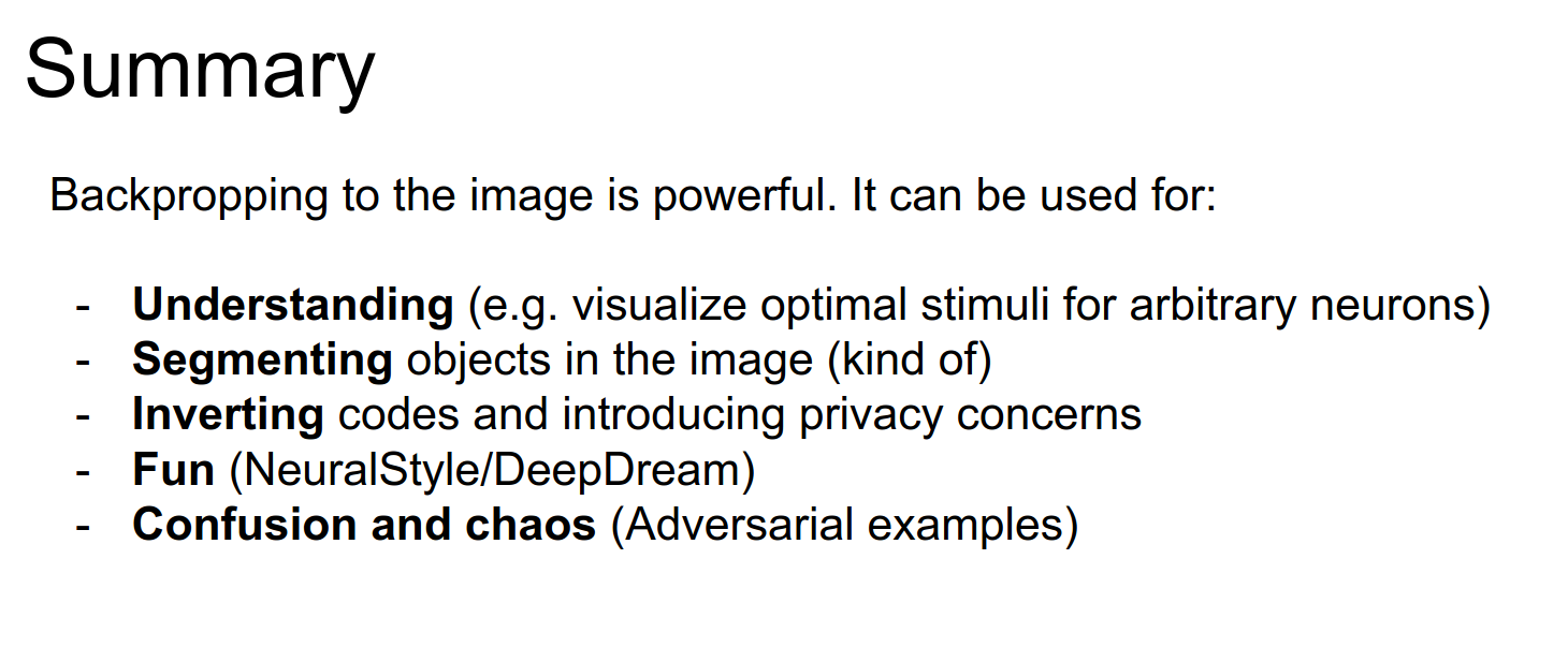
We saw that backpropping to the image can be used for understanding, segmenting, inverting, fun, and confusion.
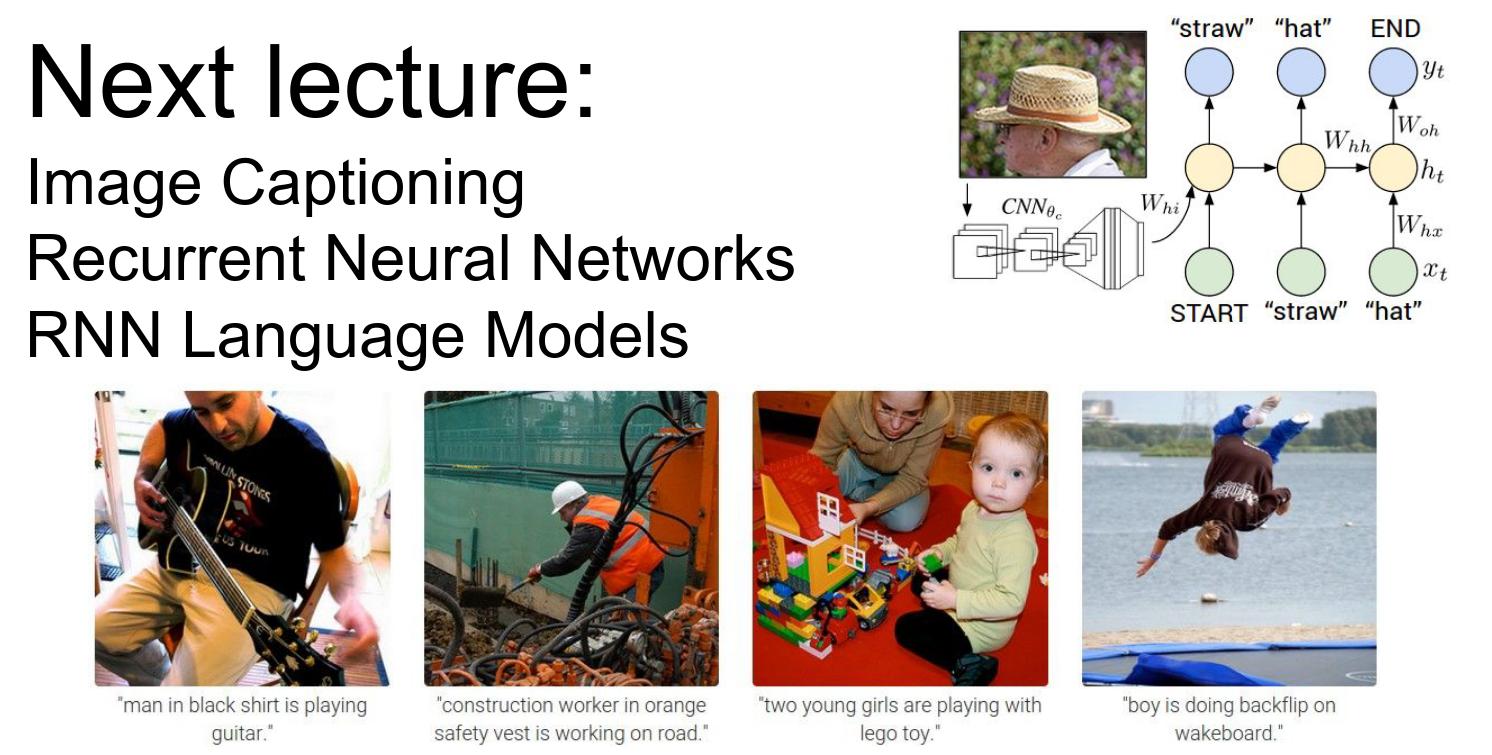
We will go into RNNs.
What are these?
What are these?
What are these?
Done with lecture 9!