10. RNNs & LSTMs

Part of CS231n Winter 2016

---

Lecture 10: Recurrent Neural Networks

Midterm coming up, A3 is going to be released.

We tried to understand Convolutional Neural Networks, saw ConvNets, Style Transfer, and Adversarial Inputs.

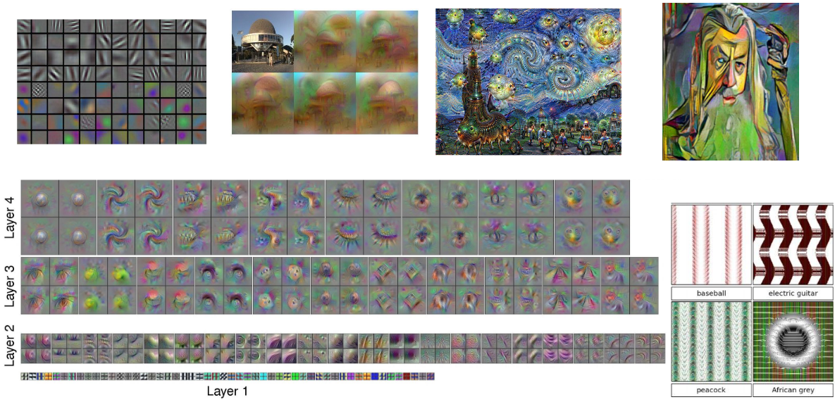
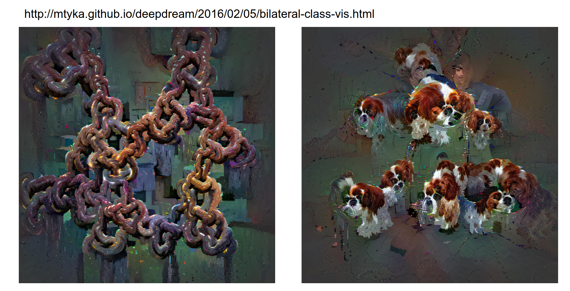
A lot of different examples here.

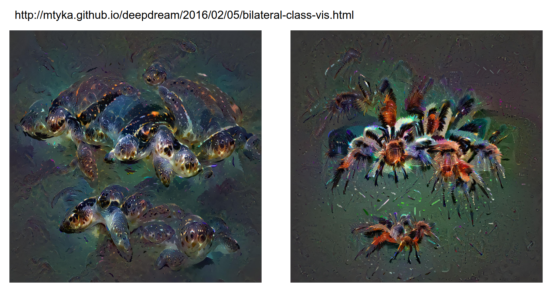
Pretty cool stuff. I think this is like DeepDream with a fancy filter.

We will talk about Recurrent Neural Networks.

RNN Flexibility

Definition

Recurrent Neural Networks, also known as RNNs, are a class of neural networks that allow previous outputs to be used as inputs while having hidden states.

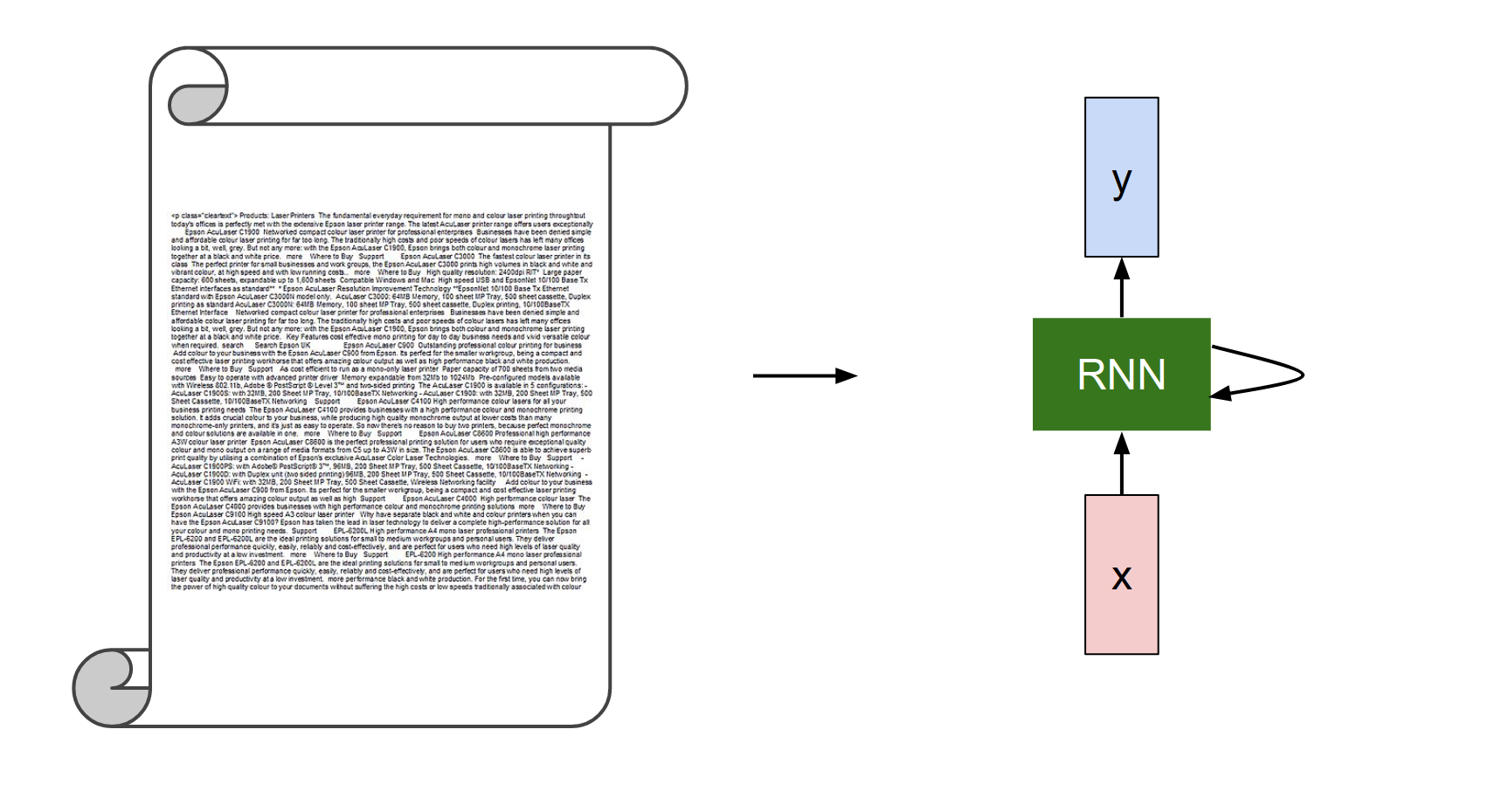
In a Vanilla NN, you have a fixed-size input (red), you process it with some hidden layers (green), and you get a fixed-size output (blue).

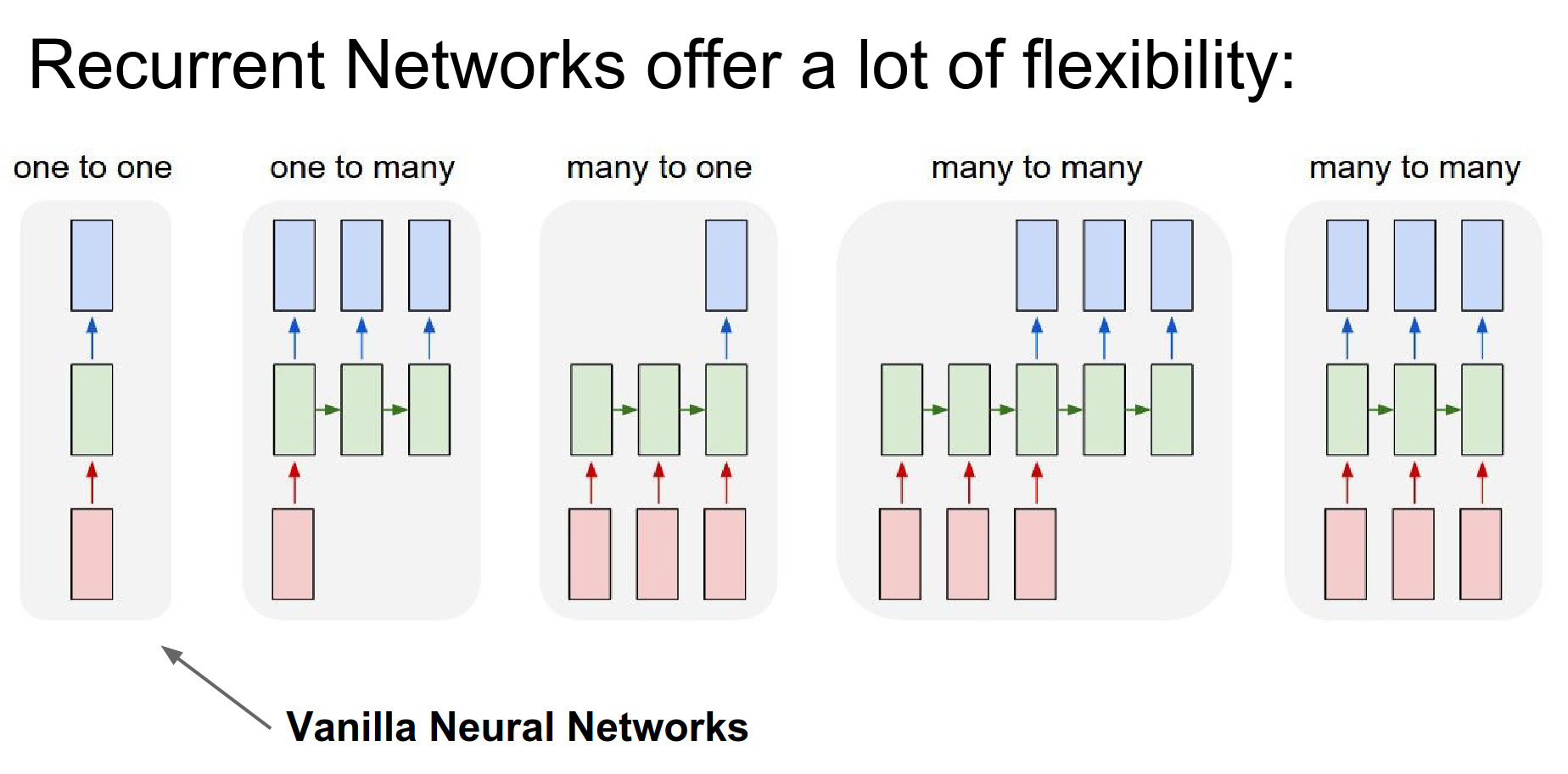
We can operate on sequences with RNNs. At the input, output, or both at the same time.

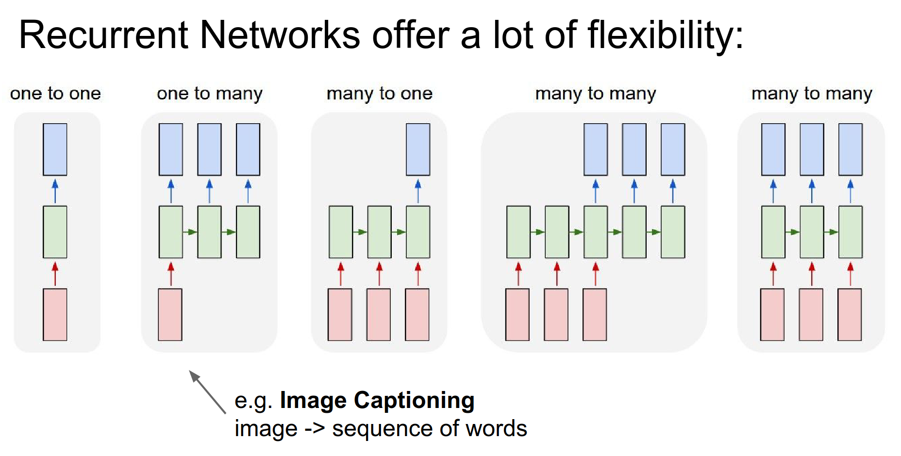
In the case of Image Captioning, you are given a fixed-size image, and through an RNN, you will get a sequence of words that describe the content of that image.

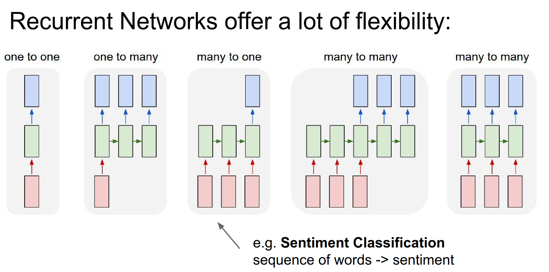
In sentiment classification in NLP, we consume a number of words in a sequence, and we try to classify whether the sentiment is positive or negative.

Seq to Seq 🌉

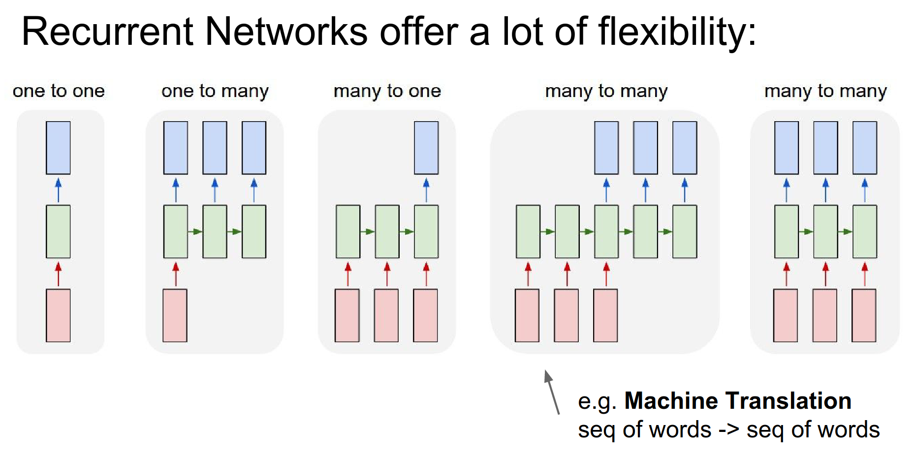
In Machine Translation, we can have an RNN that takes a number of words in English and is asked to produce a number of words in French as a translation.

Maybe we want to do video classification, classifying every single frame of video with some number of classes. We want the prediction to be made not only on a single frame but also considering the frames before it.

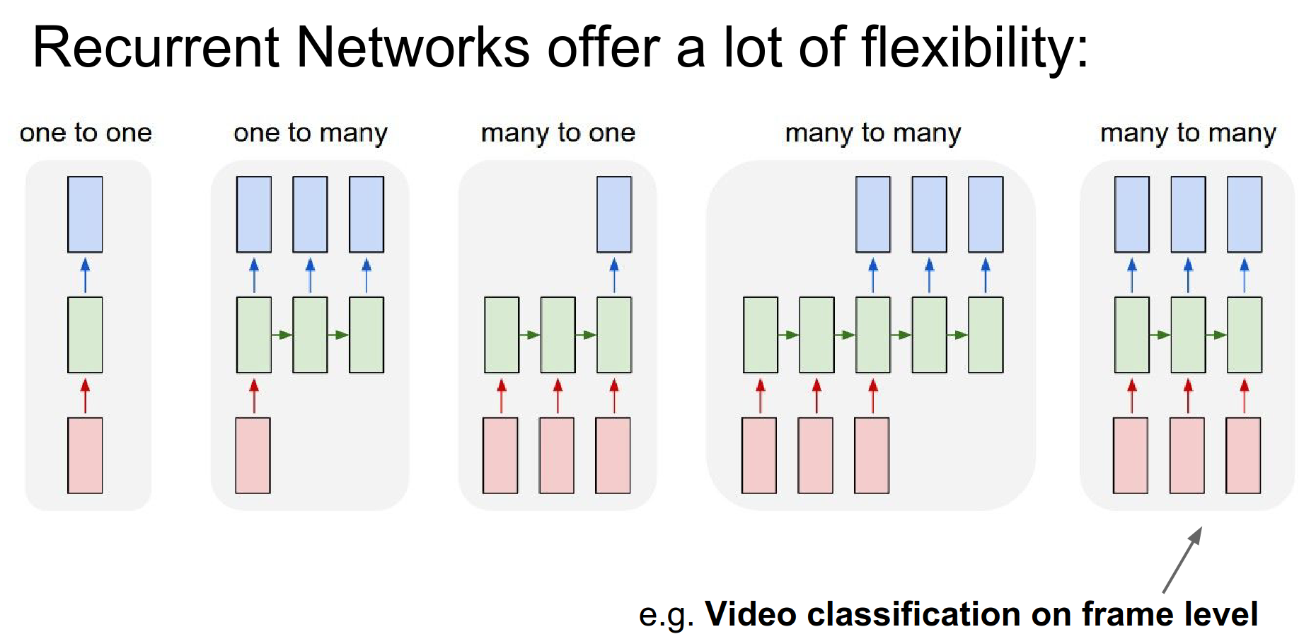
RNNs allow you to fire up an architecture where the prediction at every single timestamp is a function of all the frames that have come up until that point.

Even if you do not have sequences as inputs and outputs, you can still use an RNN, as in the case on the very left. You can process your fixed-size inputs or outputs sequentially.

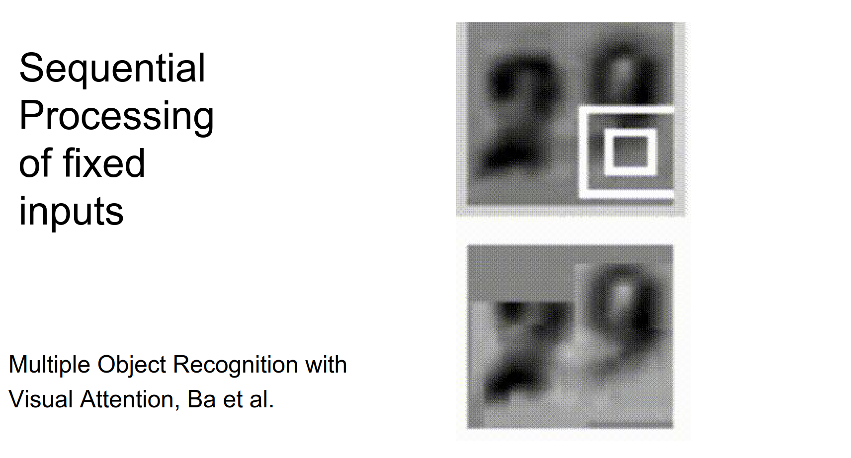
Case Study: House Numbers

Instead of just feeding a big image into a ConvNet and trying to classify the house numbers in it, they came up with an RNN policy.

A small ConvNet is steered around the image spatially with an RNN. The RNN learned to basically read out house numbers from left to right, sequentially.

So we have a fixed-size input, but we are processing it sequentially.

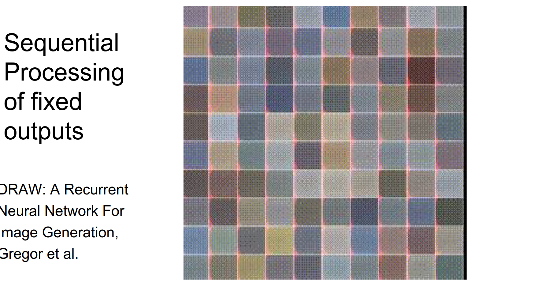
Conversely, we can think about the DRAW paper.

DRAW: A Recurrent Neural Network For Image Generation:

This is a generative model. What you are seeing are samples from the model; it is coming up with these digit samples. We are not predicting the digits at a single time; we have an RNN that treats the output as a canvas, and the RNN goes in and paints it over time.

You are giving yourself more chance to do some computation before you produce your output. It's a more powerful form of processing data.

RNN Basics

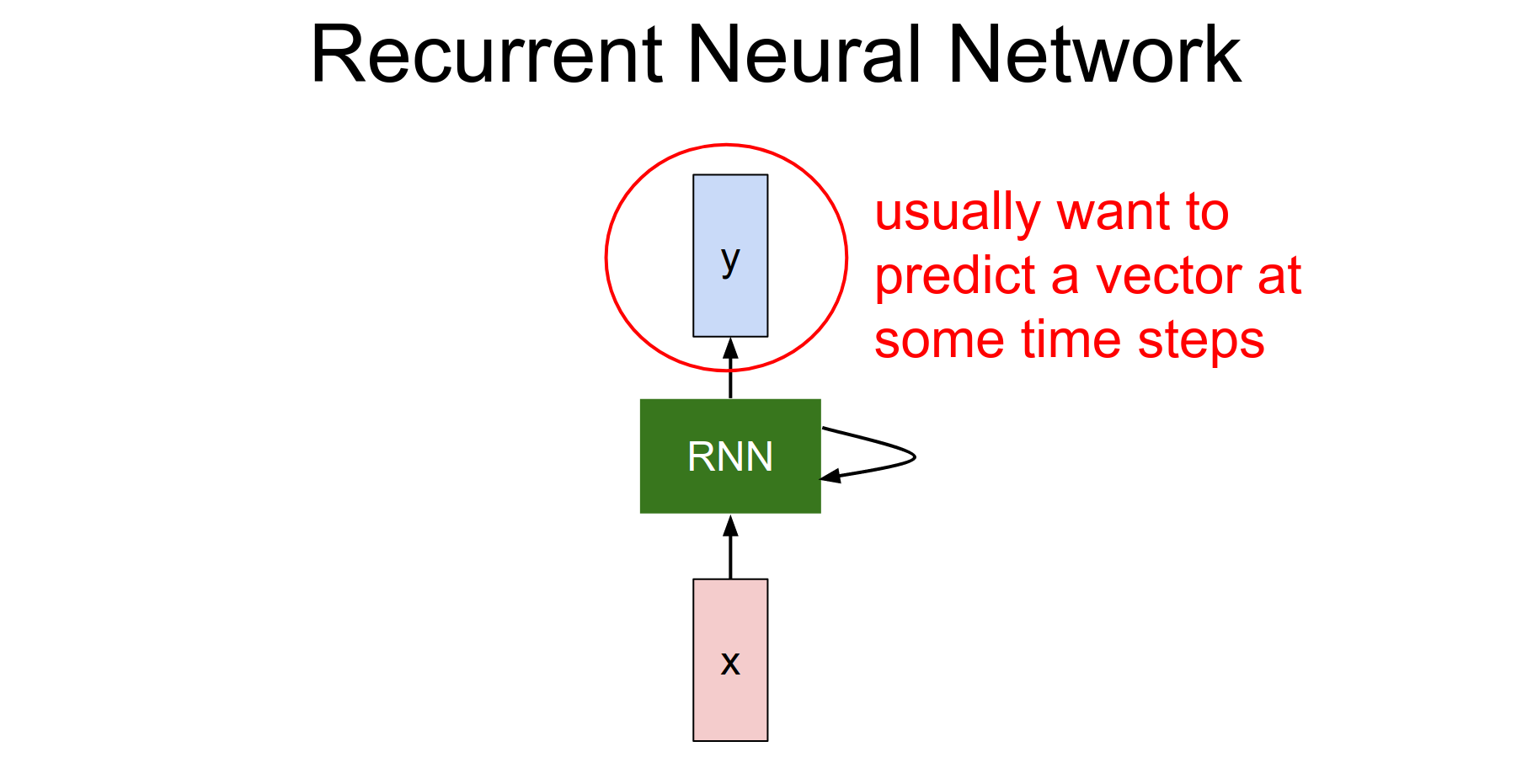
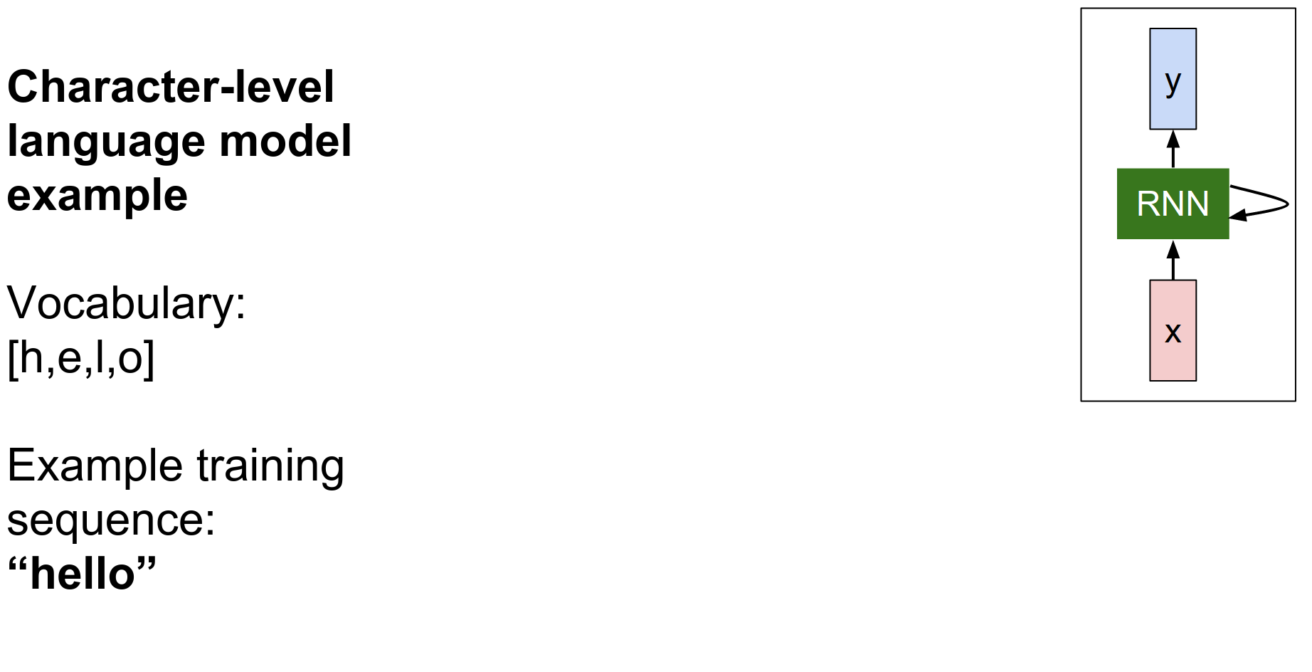
This is a box that has some internal state and receives input vectors. It can modify its state as a function of what it receives at every single timestamp.

There will be weights inside the RNN. As we tune the weights, the RNN will have different behavior in terms of how its state evolves as it receives inputs.

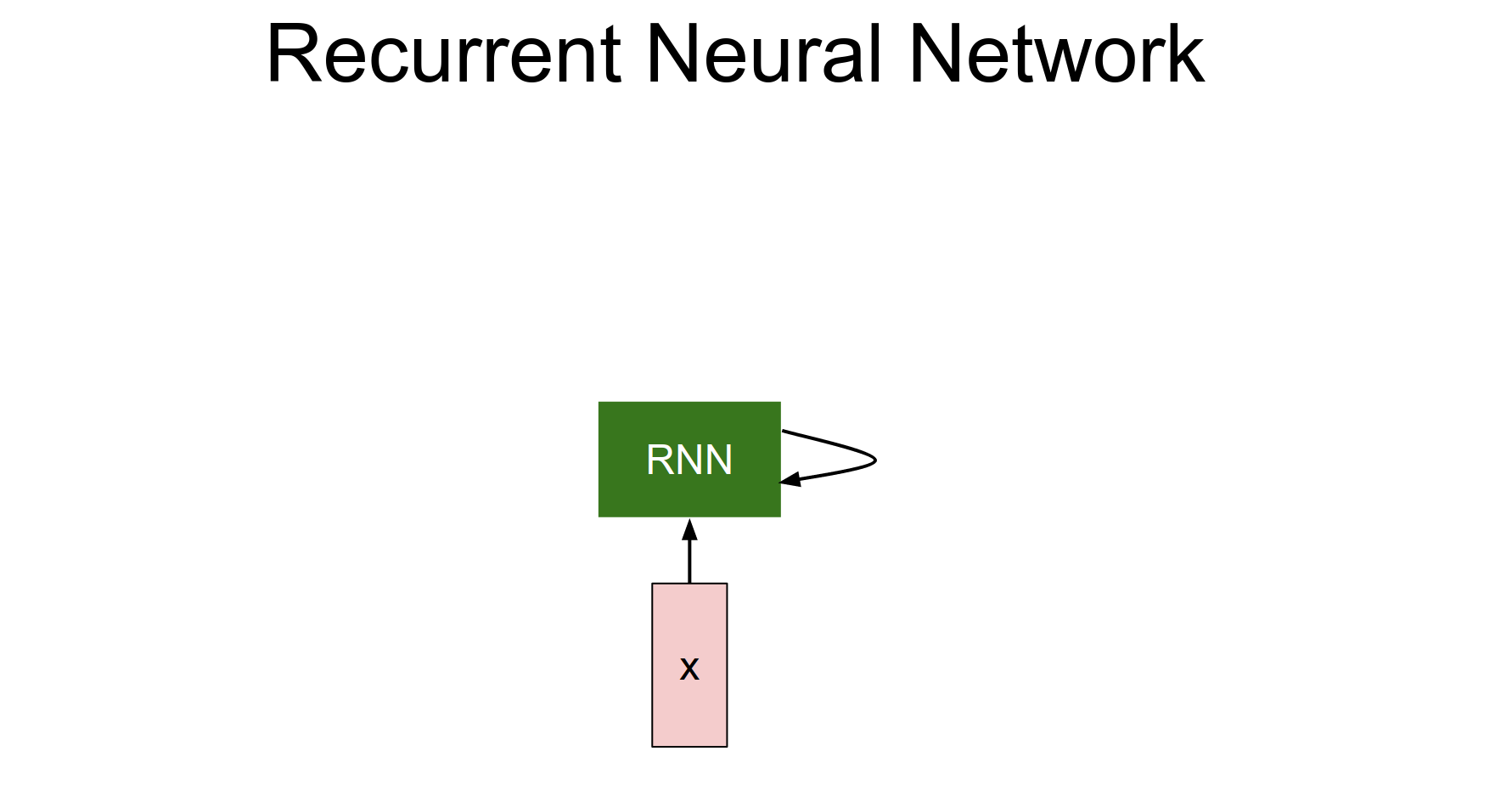
We can also be interested in producing an output based on the RNN's state, so we can produce these vectors on top of the RNN.

The RNN is just the block in the middle.

The RNN has a state vector \(h\). We are going to base it as a function of the previous hidden state \(h_{t-1}\) and the current input \(x_{t}\).

Recurrence Function

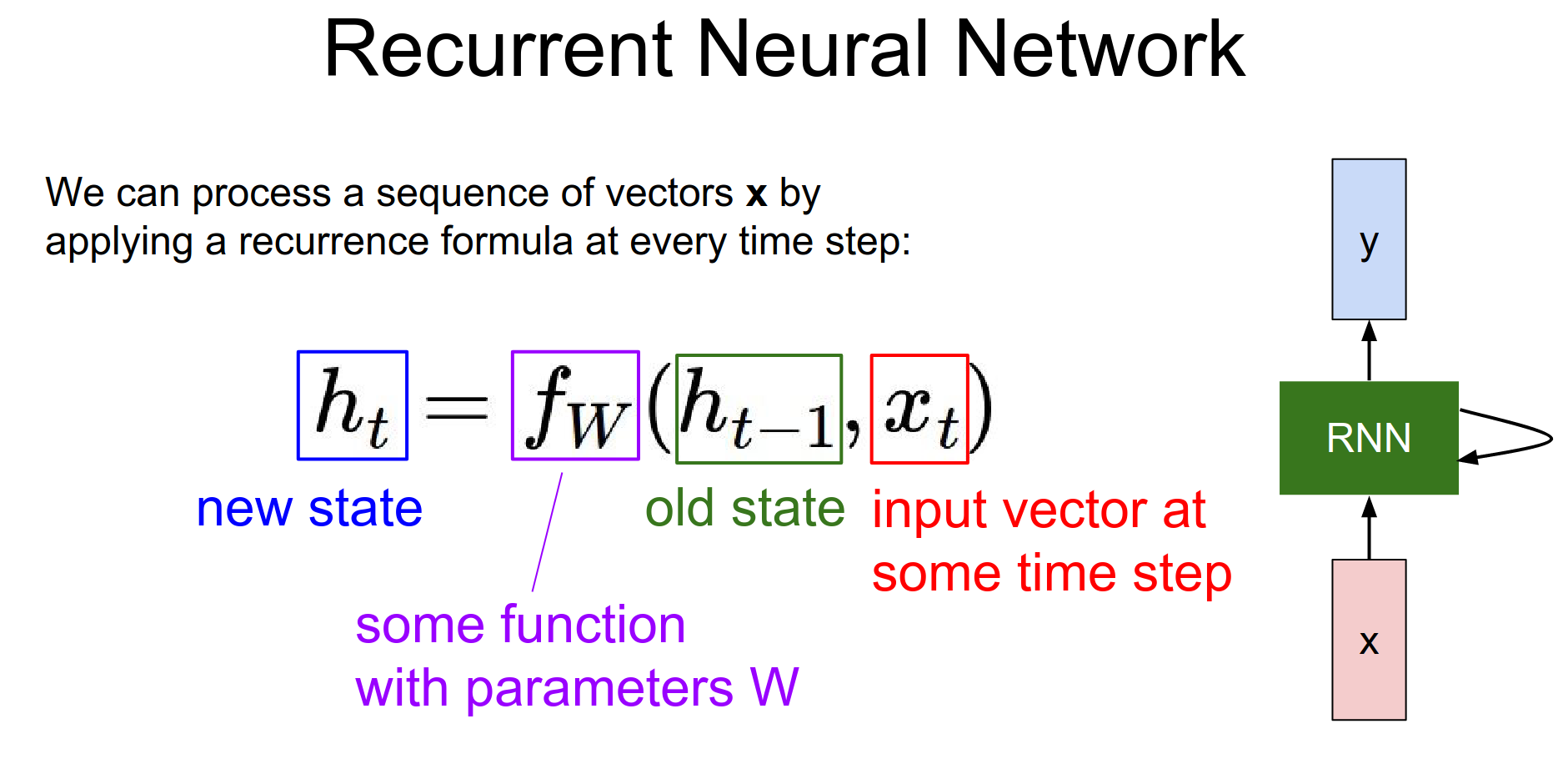
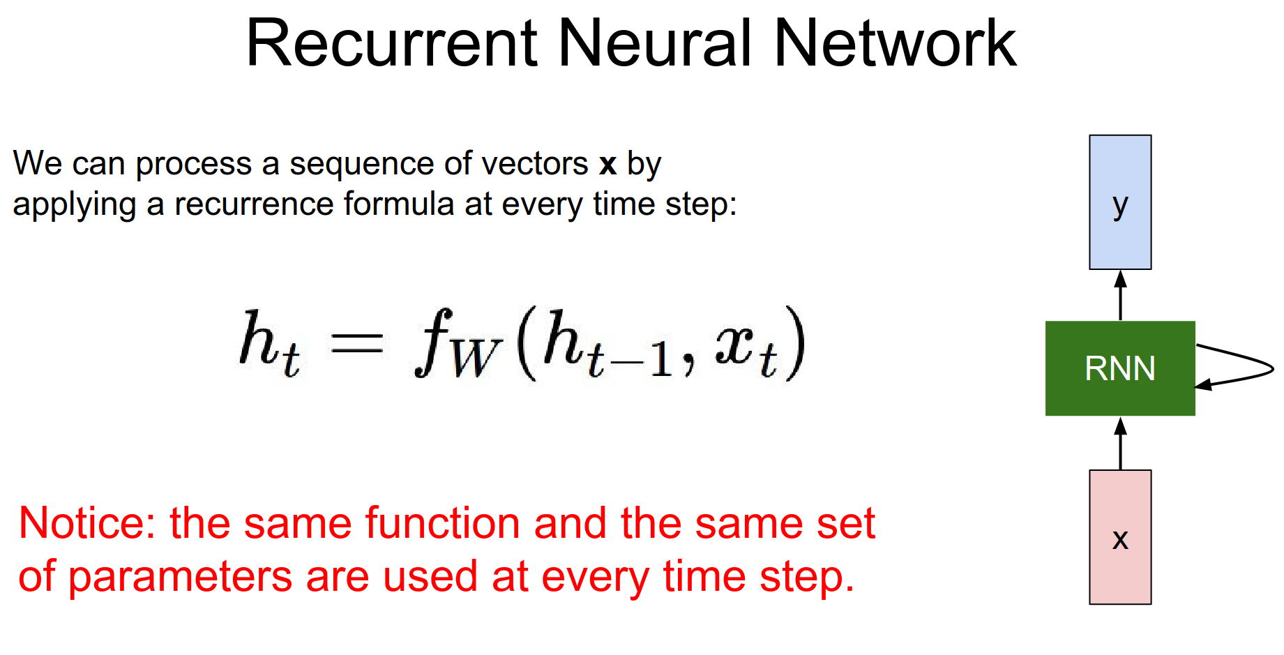
We apply the same function at every single time step. That allows us to use the RNN on sequences without having to commit to the size of the sequence.

Because we apply the same function no matter how long the input or output sequences are.

Simple RNN

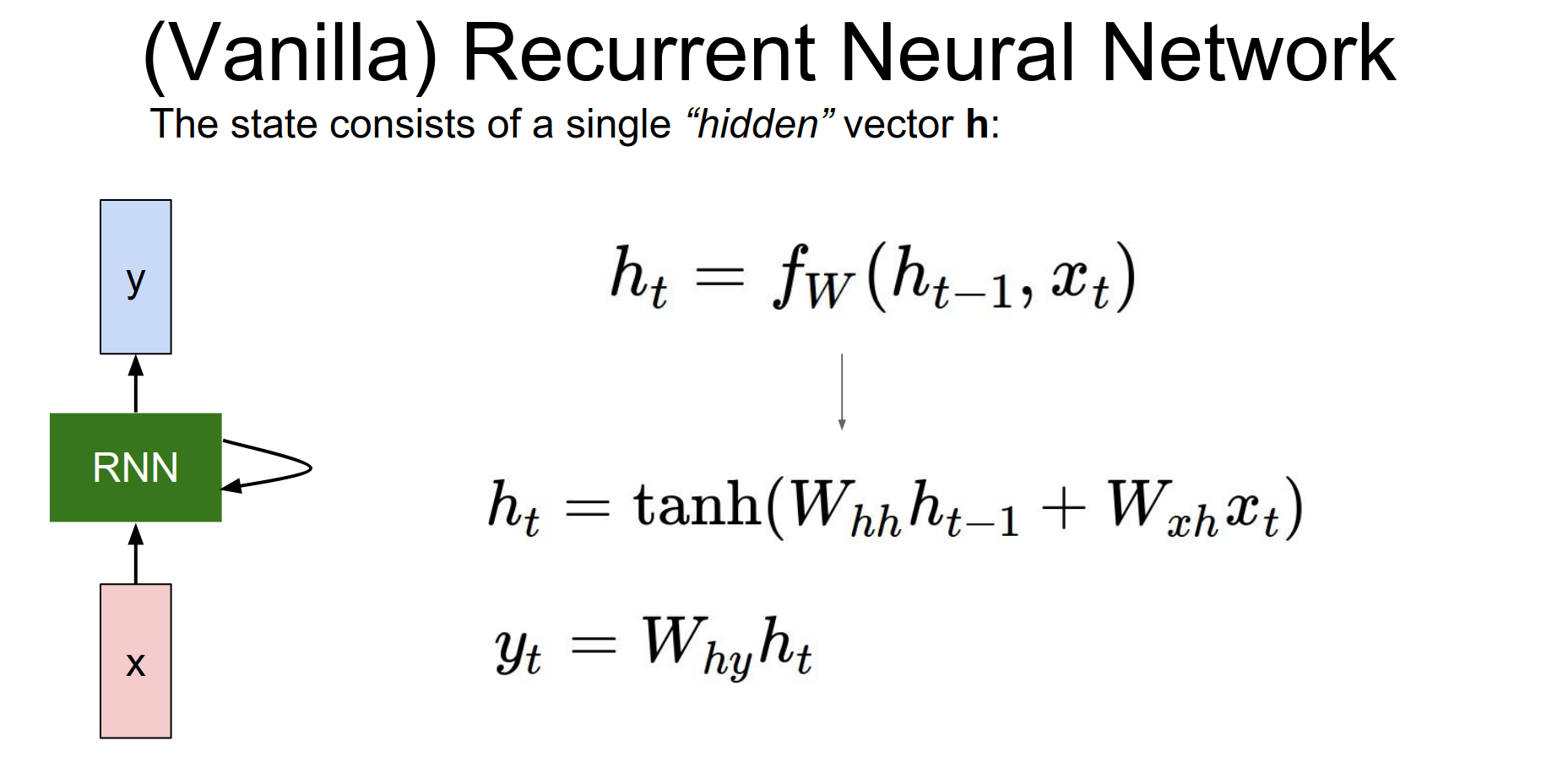
The simplest way is just a single hidden state.

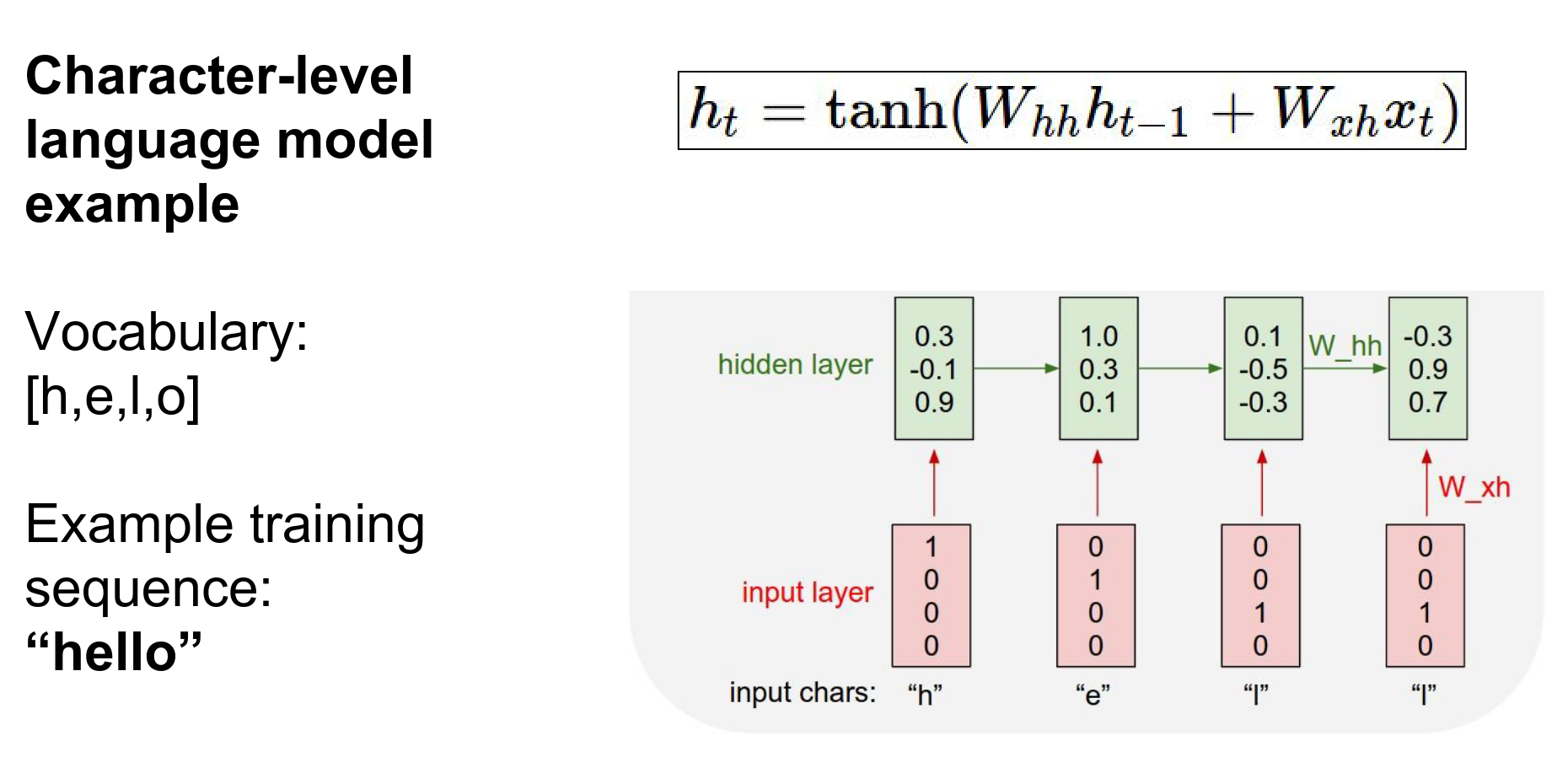
The recurrence formula tells us how we should update the hidden state \(h\) as a function of the previous hidden state and the current input \(x_{t}\).

Weight Matrices

They will project the hidden state from the previous step and the current input.

They will add, and we will squish them with a \(tanh()\).

Activation Function

That's how we update the hidden state at time \(t\).

We can base predictions on top of \(h\) using another projection on top of the hidden state.

Simple example: we will feed a sequence of characters into an RNN. At every single time step, we will ask the RNN to predict the next character in the sequence.

So we will predict an entire distribution of what it thinks should come next in the sequence that it has seen so far.

We will feed all characters one at a time, encoding characters with One-Hot Representation.

One-Hot Encoding 🥰

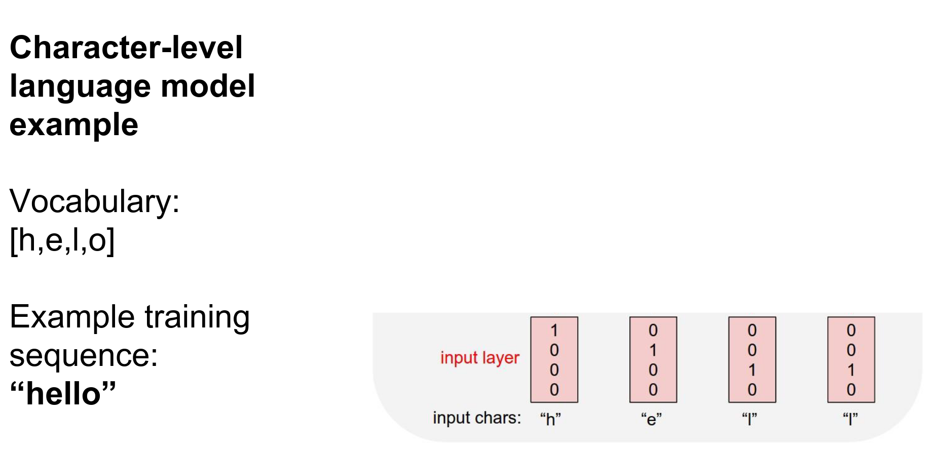
We will use the recurrence formula. Suppose we started with \(h\)'s at all zero.

We use the same recurrence formula at every step to update the hidden state with the sequence it has seen until then.

We will predict at every single time step what the next character in the sequence should be.

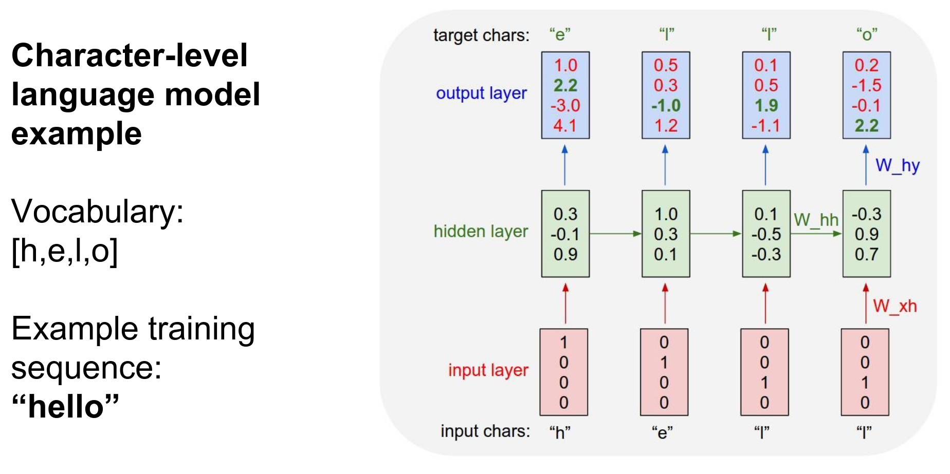
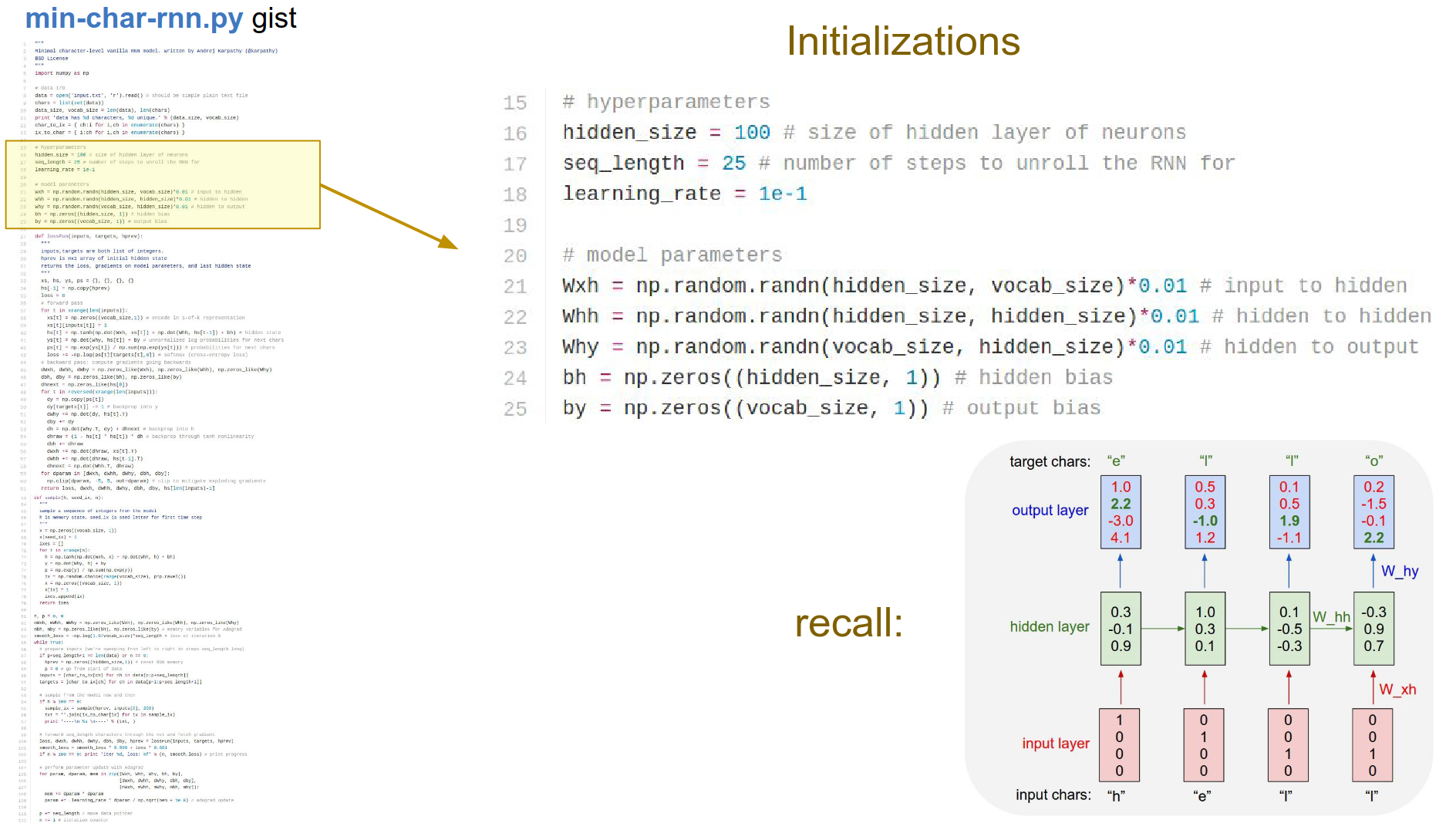
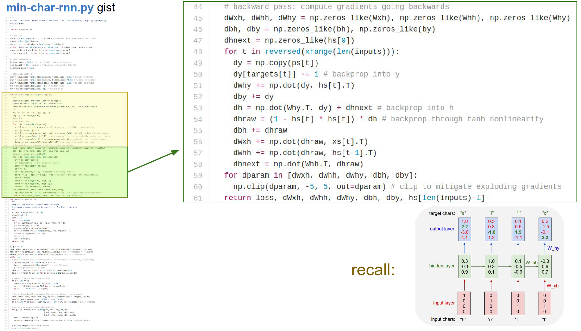
For example, in the very first time step, the RNN computed unnormalized log probabilities: It thinks:

• \(h = 1\)
• \(e = 2.2\)
• \(l = -3\)
• \(o = 4.1\)

are likely right now.

We want "\(e\)" to be high and all the other numbers to be low.

In every single time step, we have a ==target== for what the next character should be in the sequence. That is encoded in the gradient signal of the loss function. That gets backpropagated through these connections.

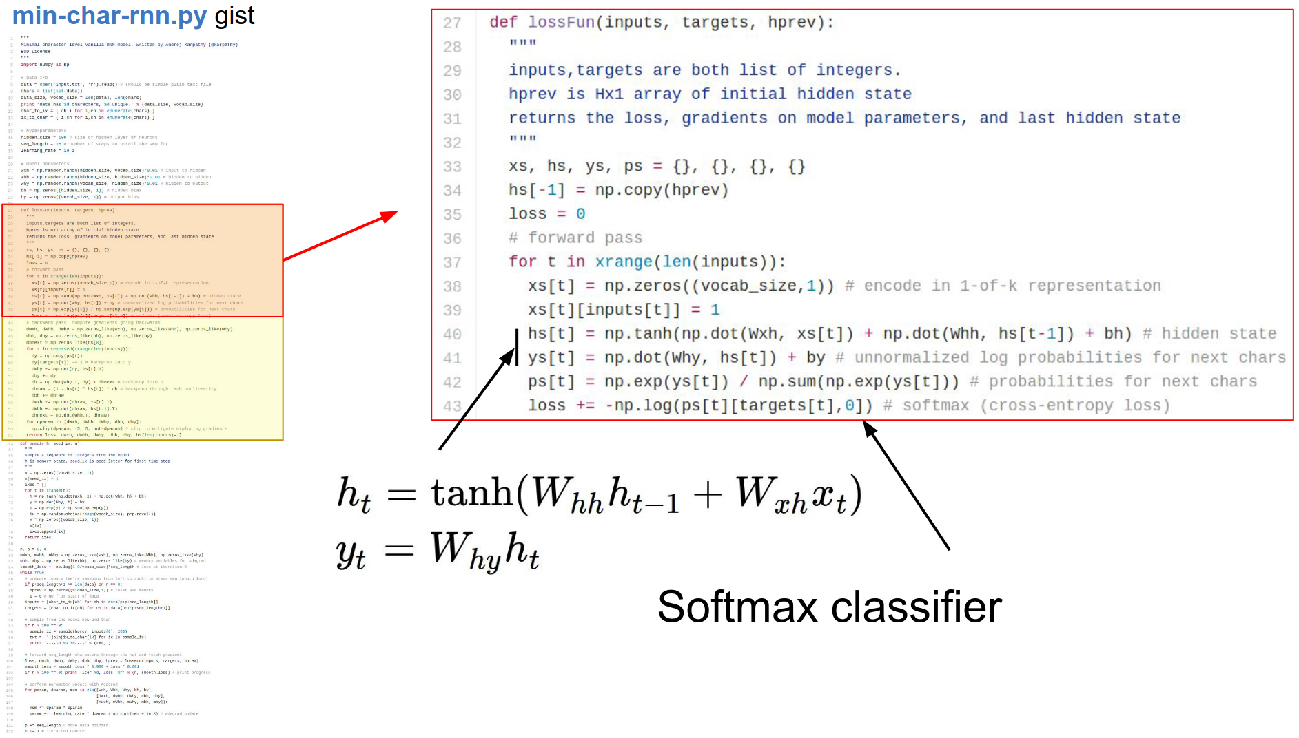
Another way to think about it: at every single time step, we have a softmax classifier over the next character, and at every single point, we know what the next character should be.

We get all the losses flowing down from the top. They will all flow through this graph backwards through all the arrows. We are going to get gradients on the weight matrices, then we will know how to shift the matrices so that the correct probabilities are coming out of the RNN.

We will be shaping the weights so that the RNN has the correct behavior as we feed in data.

At multiple time steps, we use the same \(W\)'s. In backpropagation, you have to consider this. This allows us to process variably sized inputs because at every time step we are doing the same thing; we are not a function of the absolute amount of things in the input.

Initialization

First \(h == 0\) -> initially. This is common.

Sequence Order

If this was a longer sequence, the order always matters. The hidden state depends on everything it has seen, so the order matters.

Character-Level RNN 🎈

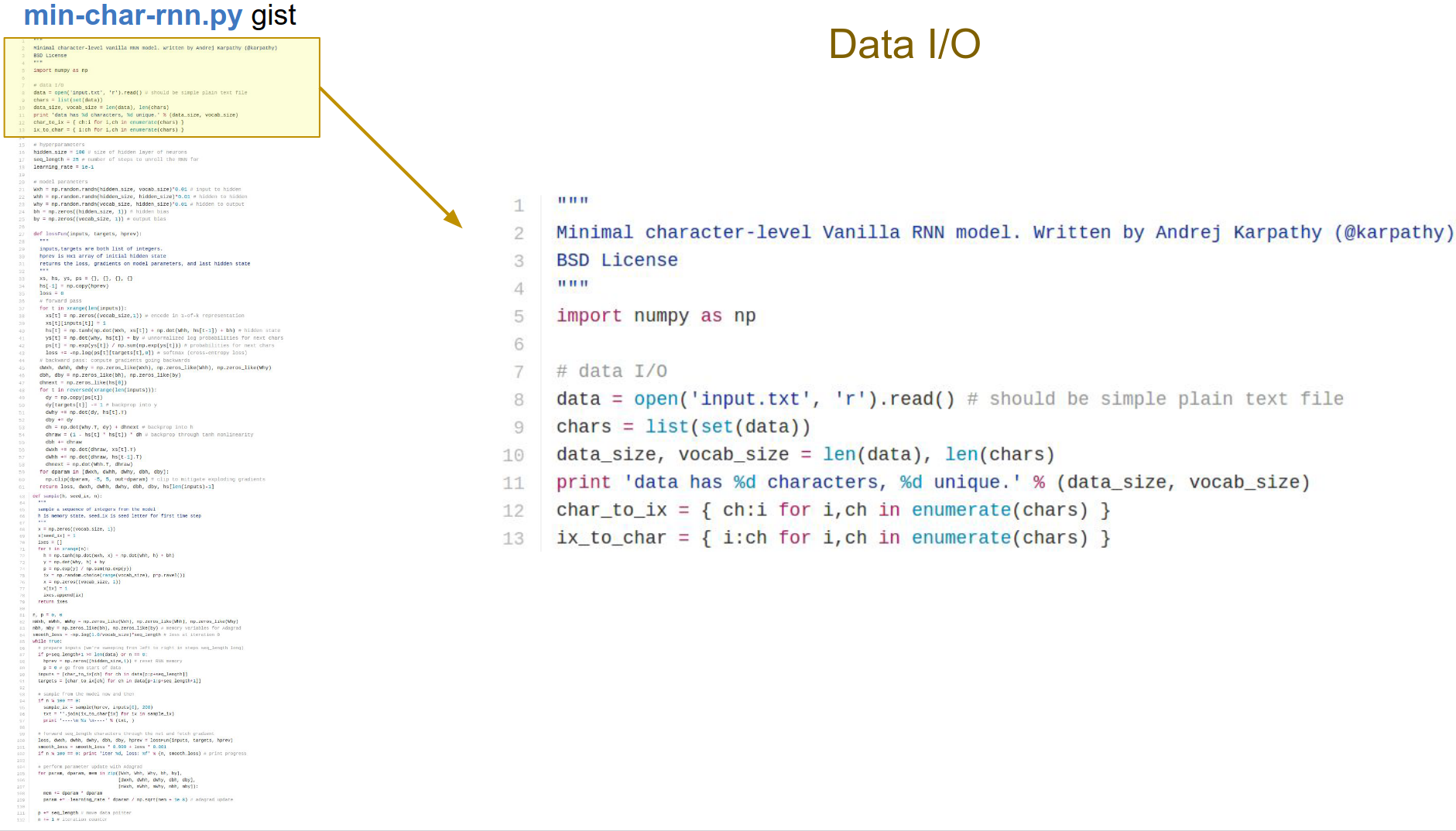
The char-rnn gist link is here. Let's work on it.

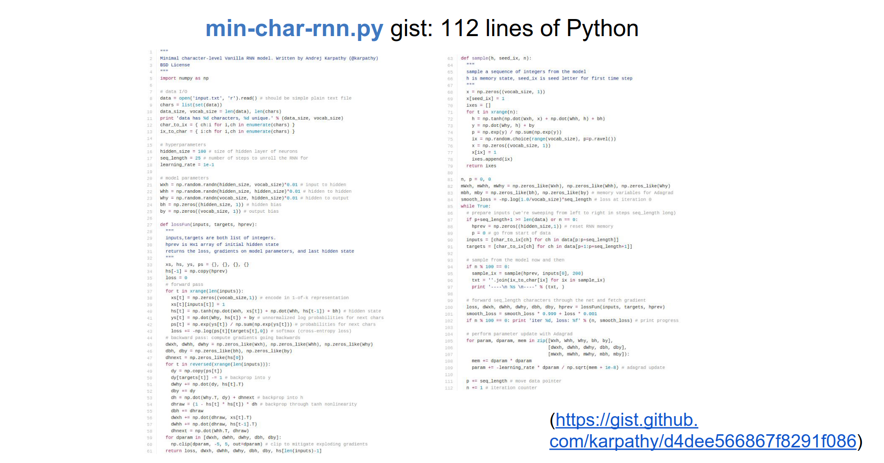
The only dependency is numpy. The input is a large sequence of characters.

We find all the unique characters and make these maps for characters to indices and indices to characters.

Our hidden_size is a hyperparameter. Learning rate is also one.

seq_length -> if the sequence is too large, we won't be able to keep it all in memory and run backpropagation on it.

We will be going with chunks of \(25\). We cannot afford to do backpropagation for longer because we would have to remember all that stuff.

We have all the \(W\) matrices and biases \(b\), initialized randomly. These are all of our parameters.

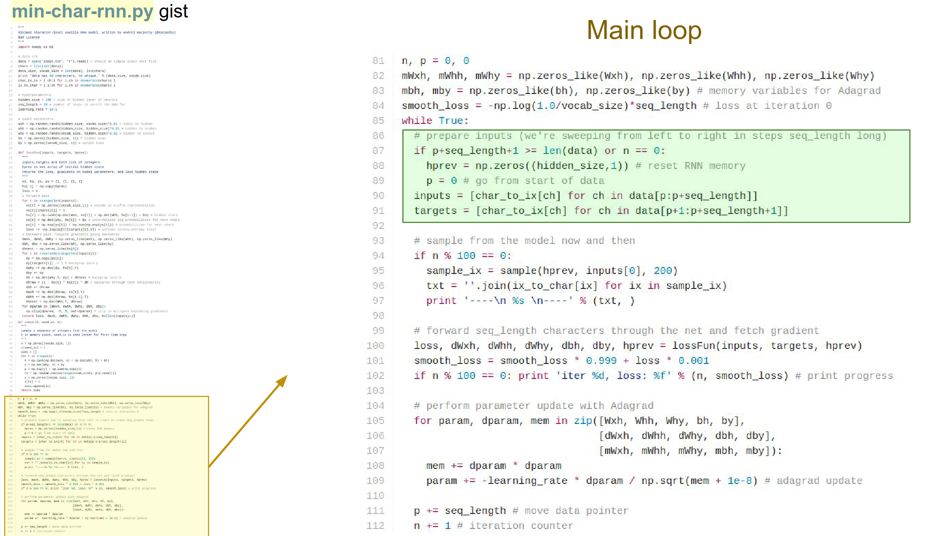
Skip the loss function for now; get to the main loop.

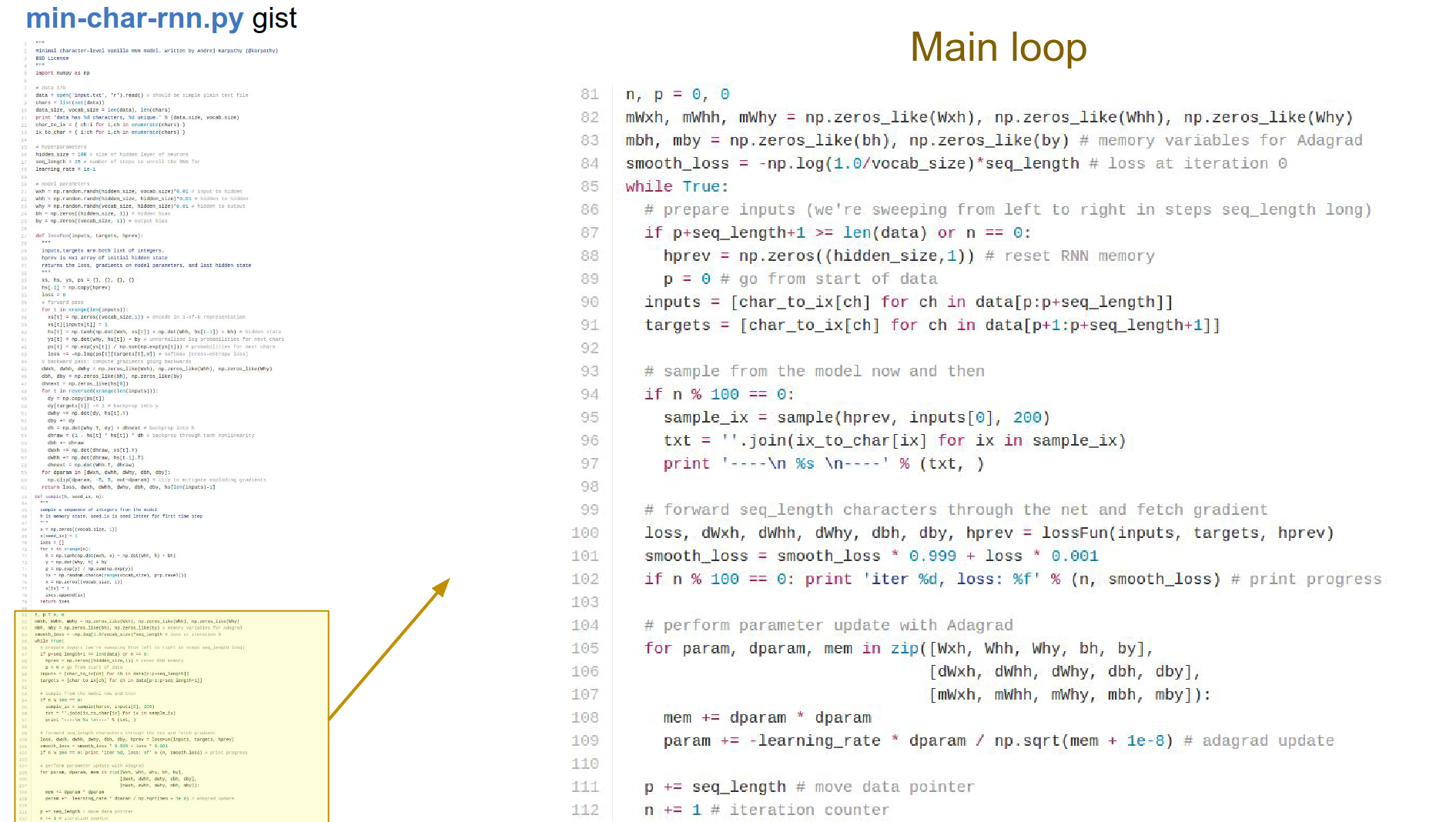
Some initializations.

We are looping forever:

• Sample a batch of data. 25 integers -> inputs list.
• targets are offset by 1 into the future.

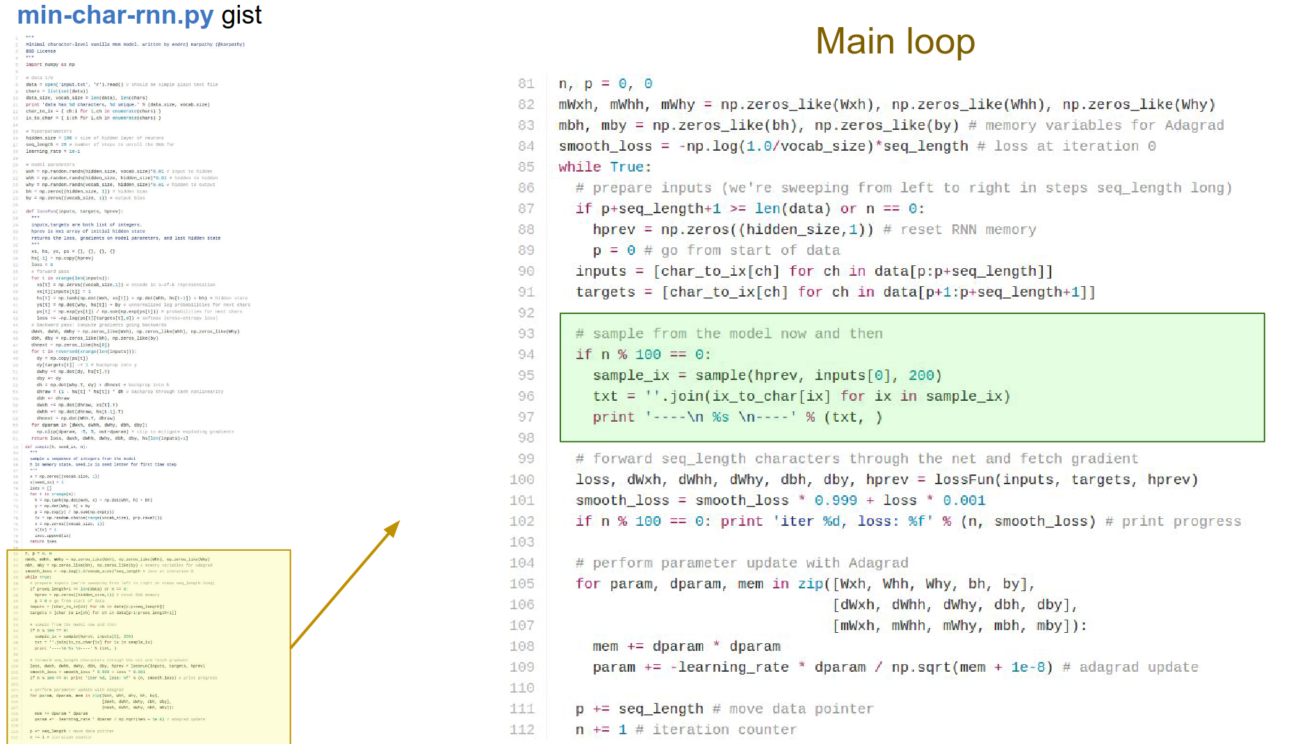
Sampling code. What do the sequences look like?

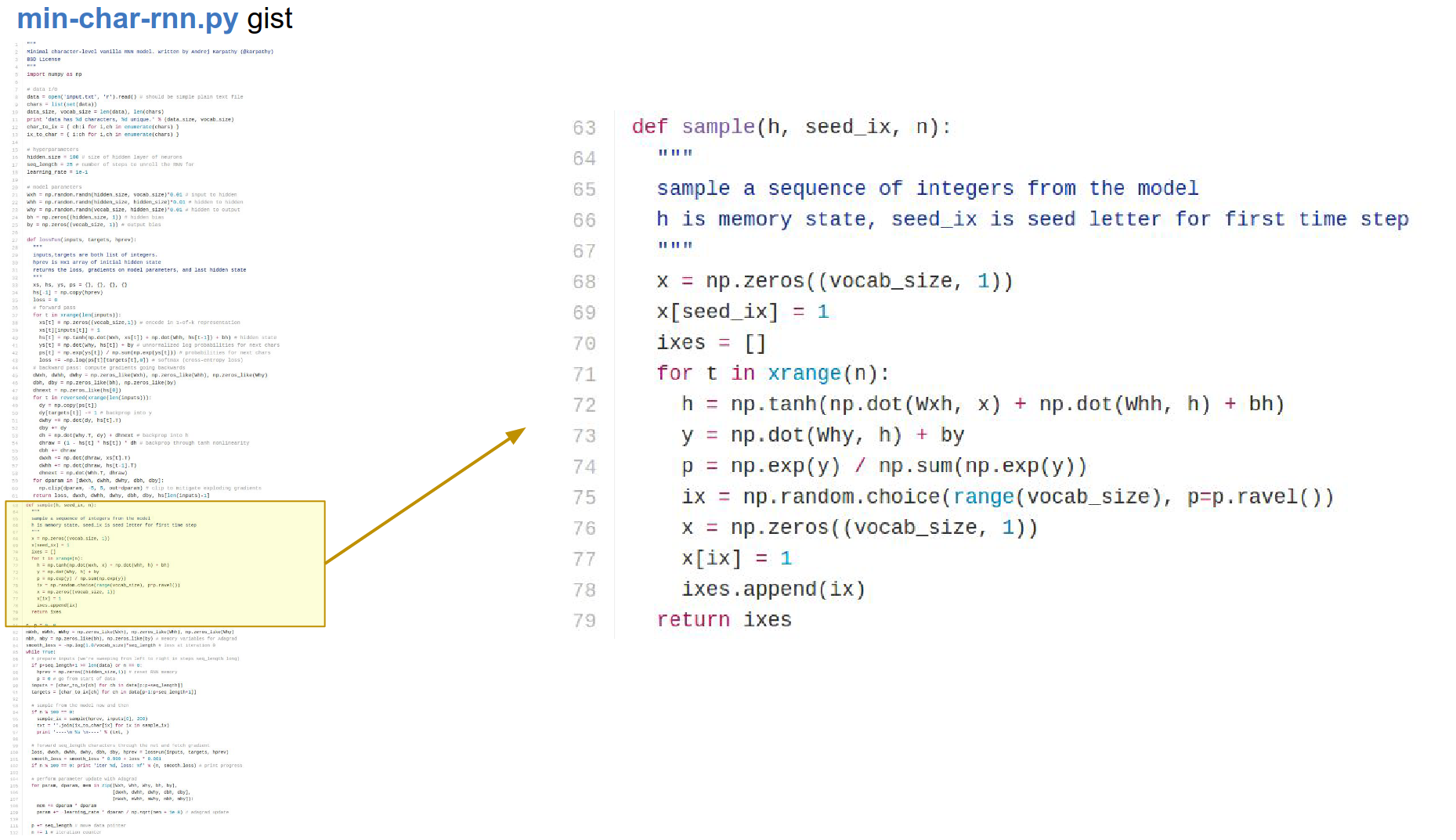
In test time, we are going to seed it with some characters. The RNN always gives us a distribution of the next character in the sequence. You can imagine sampling from it, and then you feed in the next character again.

You keep feeding all the samples into the RNN, and you can just generate arbitrary text data. It calls the sample_ix function; we will go to that in a bit.

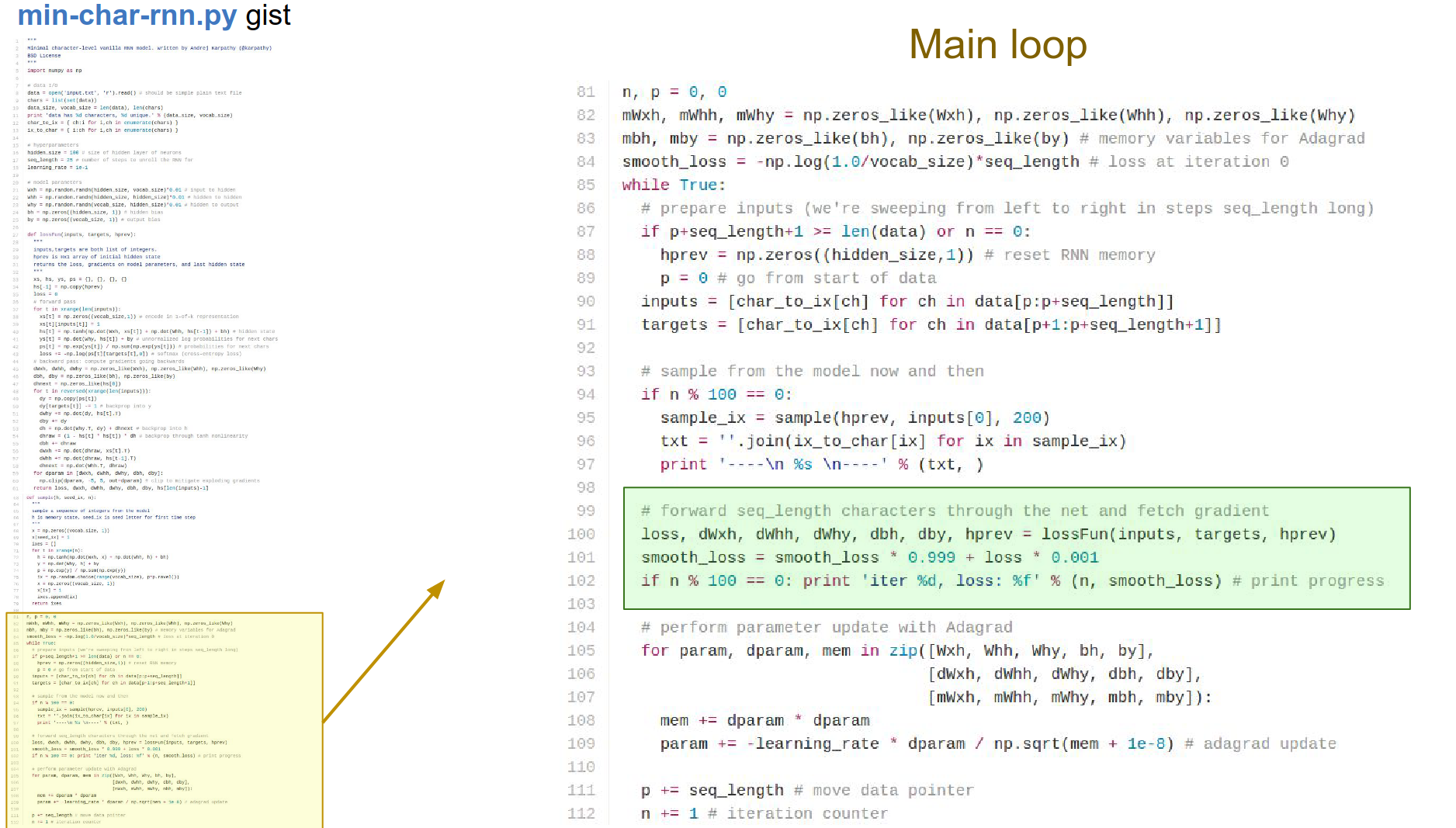
The loss function receives the inputs, targets, and h_prev. Hidden state vector from the previous chunk.

What is the hidden state vector at the end of your 25 letters? When we feed in the next batch, we can use this!

We are only backpropagating those 25 time steps.

We get the loss and gradients in all the weight matrices and the biases. Just print the loss.

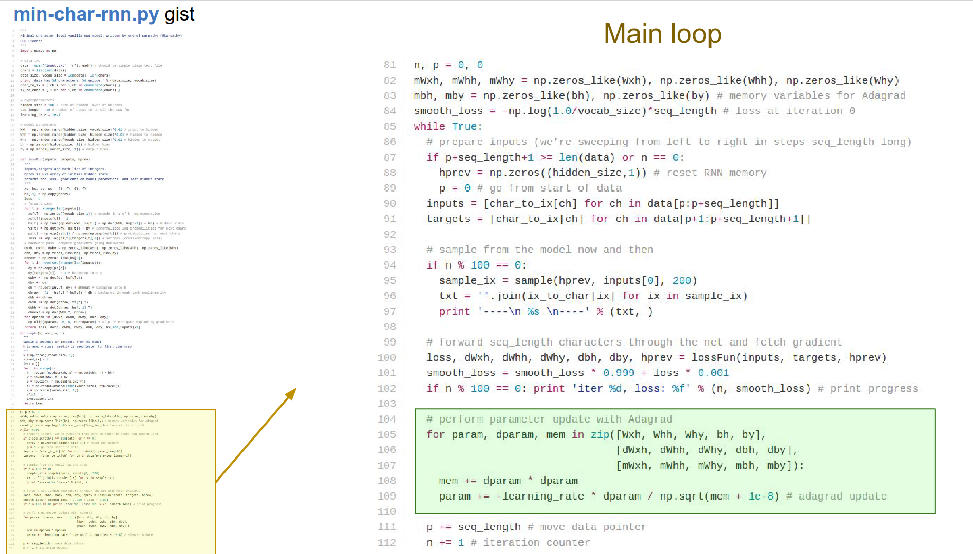
Parameter update: we know all the gradients.

Perform the update. This is Adagrad update. We have all these cached variables for the gradient squared which we are accumulating and using.

This is the loss function. Forward and Backward pass.

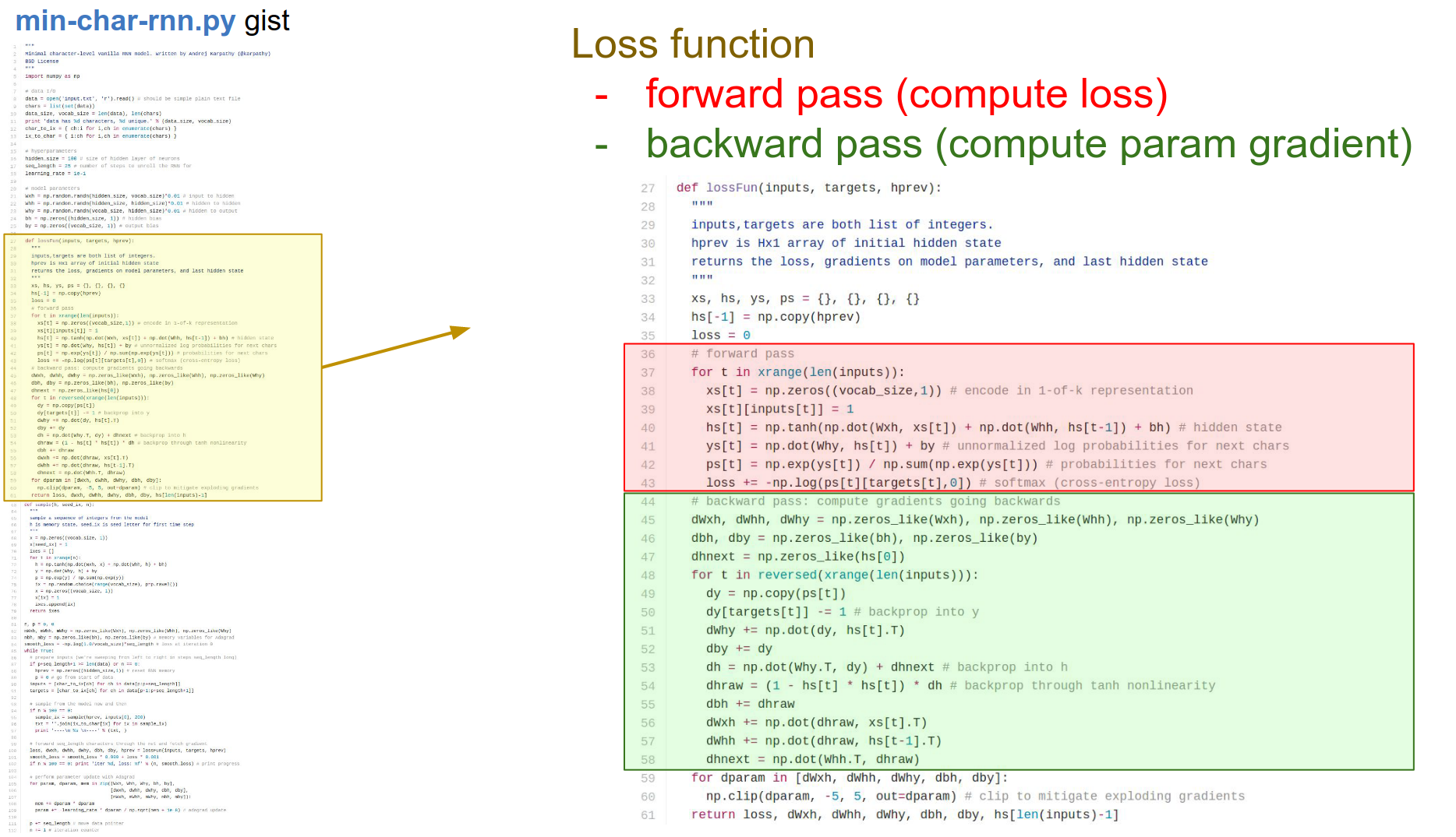
In the forward pass, you should recognize that we get inputs, targets, and hprev. We received these 25 indices, and we are now iterating through them from 1 to 25.

We make this x input vector (which is just zeros). We make one-hot encoding.

Whatever the index on the input is, we turn that bit on with a \(1\).

We are feeding into the character with a one-hot encoding, then we will compute the recurrence formula.

hs[t], ys[t], ps[t] -> Using dictionaries to keep track of everything.

We compute the hidden state vector and the output.

Compute the softmax function -> normalizing this so we get probabilities.

The last line is just a softmax classifier -> \(-log()\).

Now we will backpropagate through the graph.

In the backward pass, we will go backwards from that sequence. We will backpropagate through a softmax, backpropagate through the activation functions, backpropagate through all of it.

We will just add up all the gradients and all the parameters.

One thing to note: gradients on weight matrices like whh use a += because at every single time step all of these weight matrices get a gradient, and we need to accumulate all of it into all the weight matrices.

Because we are going to keep using all these weight matrices at every time step. So we just backprop onto them over time.

That gives us the gradients; we can use that in the loss function and perform parameter update.

Here we finally have a sampling function.

Here is where we try to actually get the RNN to generate new text data based on what it has seen and based on the statistics of the characters, how they follow each other.

• We initialize with some random character.
• We go on until we are tired.
• We compute the recurrence formula.
• Get the probability distribution.
• Sample from that distribution.
• Re-encode in one-hot representation.
• Feed it in at the next time step.

Regularization Note

Why no regularization? Andrej thinks it is not common in RNN's - sometimes it gave him worse results.

Language Agnostic

This RNN does not know anything about words or language.

We can now take a whole bunch of text and feed the RNN with it 🐤

We can take all of Shakespeare's works, concatenate all -> Just a giant sequence of characters.

At first, the RNN has random parameters and will just produce garble in the end.

When you train more, there are things like spaces, there are words, it starts to experiment with quotes, it basically learned various short words!

When you train with more and more, it learns to close quotes, it learns to end sentences with a dot.

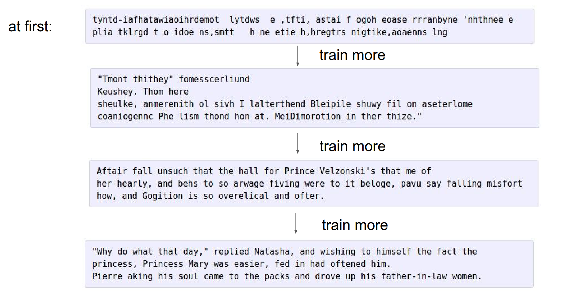
Here is an example below.

Long-term Dependencies 🤔

They fed it with a .tex file.

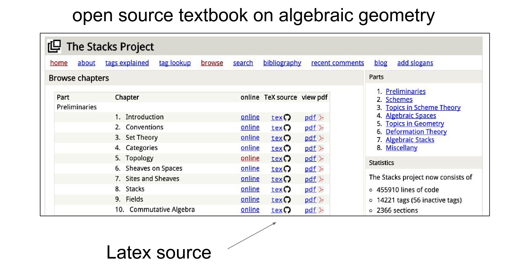
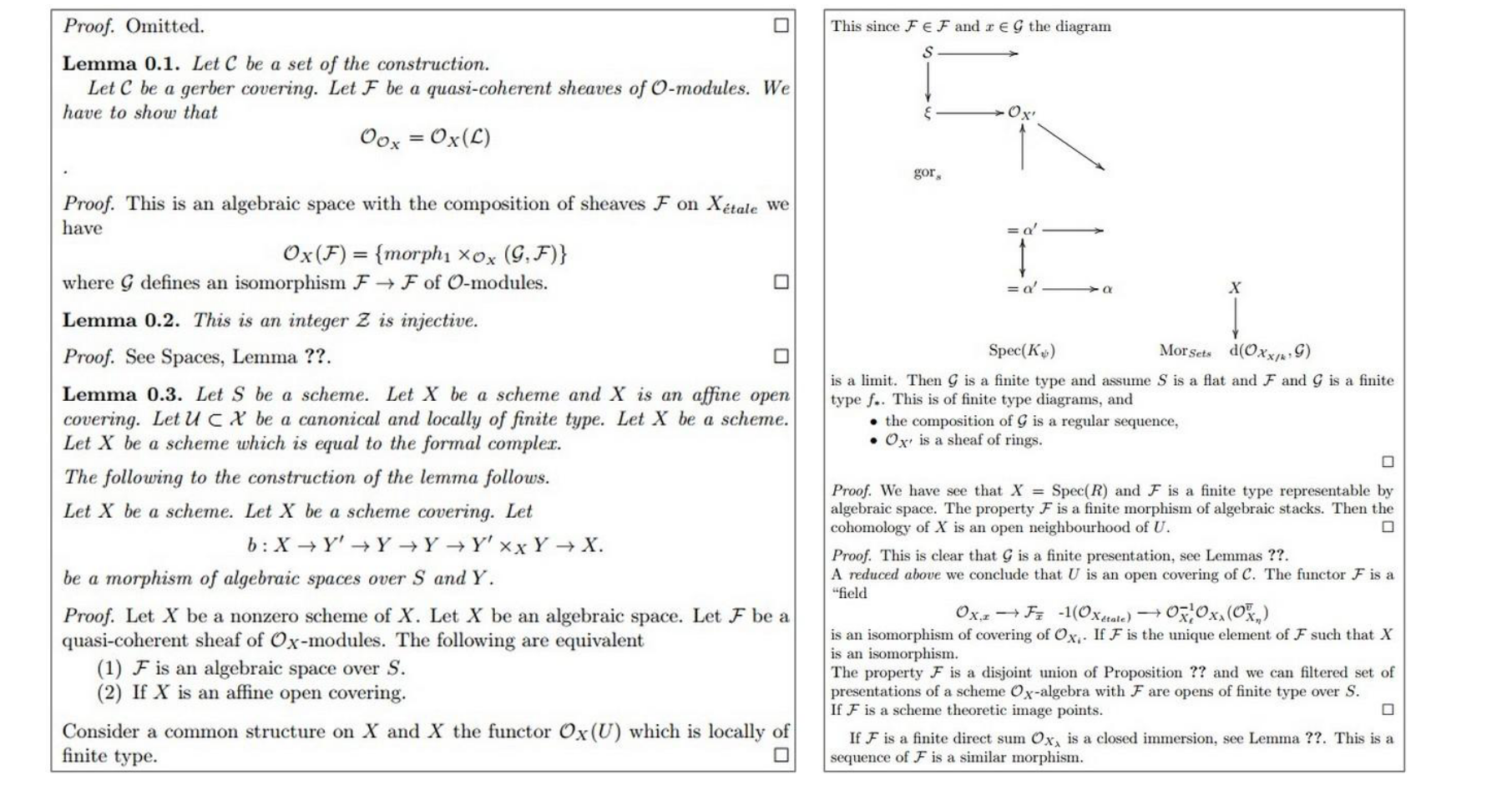
RNN can learn to generate mathematics! ->

RNN spills out LaTeX. It does not compile it right away; we had to tune it, but then voila!

It knows to put squares at the end of proofs, it makes lemmas, etc.

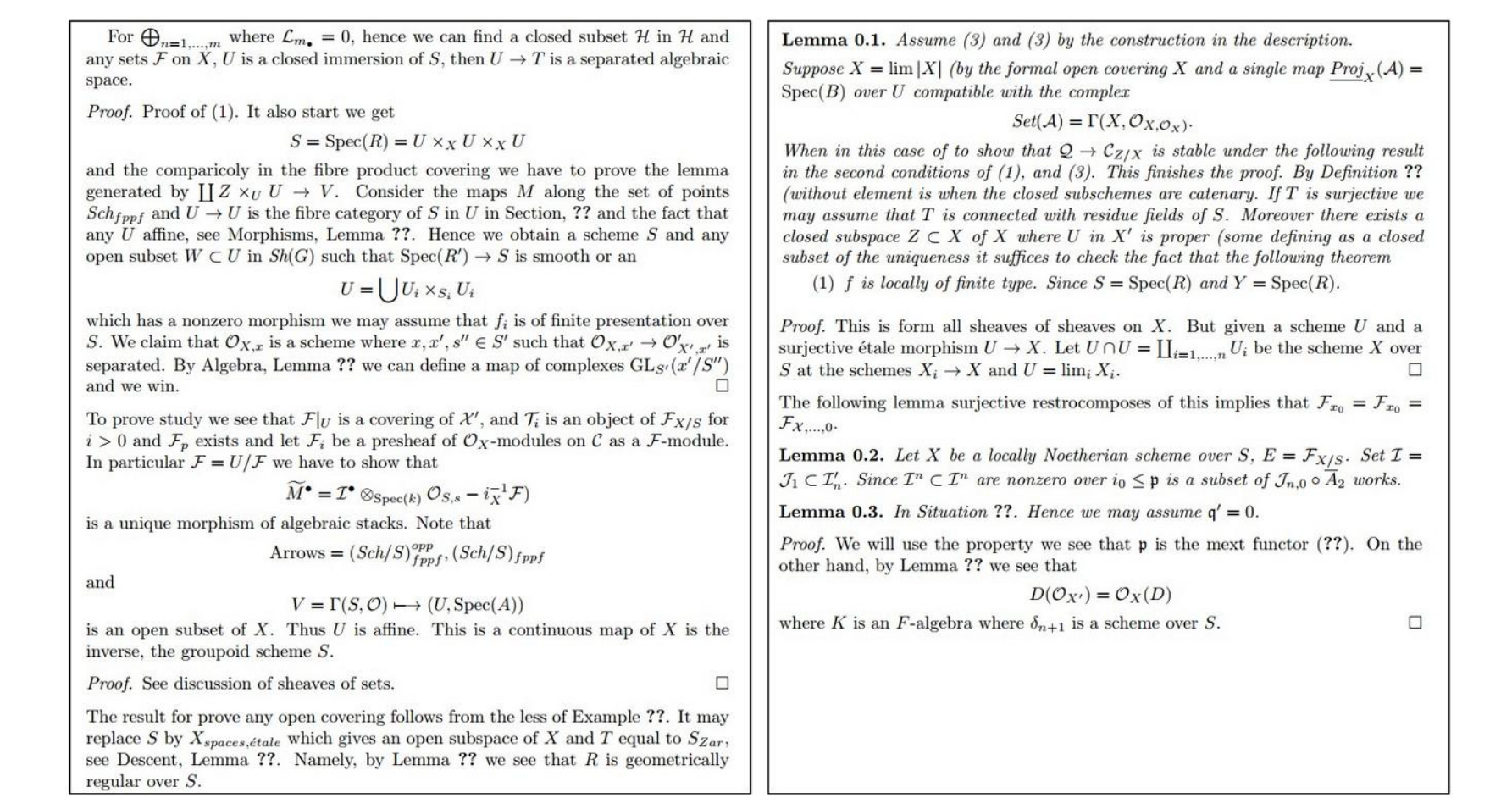
Sometimes it tries to make diagrams, but with varying amounts of success! 😅

Proof Omission - Proof. Omitted. LOL

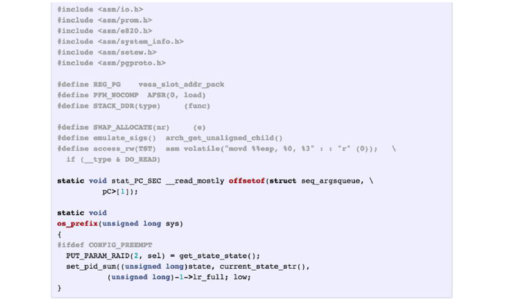
The source code is really difficult -> 700 MB of just C code and header files.

It can generate code.

Syntax-wise it makes very few mistakes. It knows about variables, it knows indentation, it makes bogus comments LOL.

It declares variables that it never ends up using. It uses variables never declared.

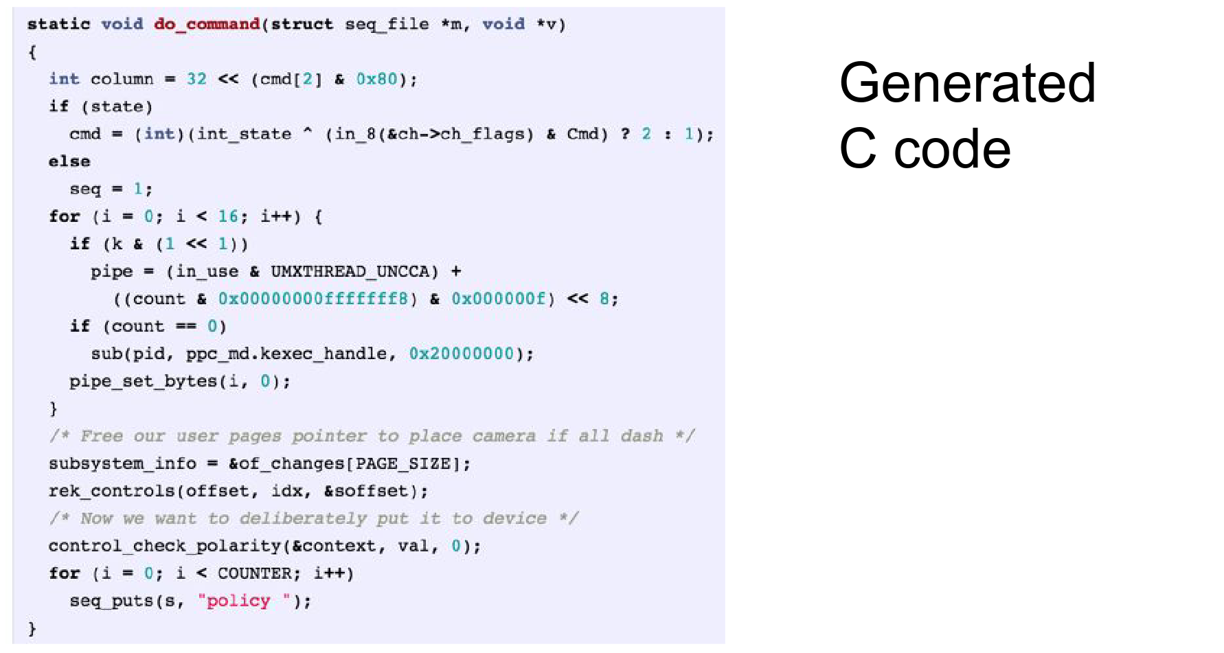
It knows how to cite, GNU license character by character. 🥳

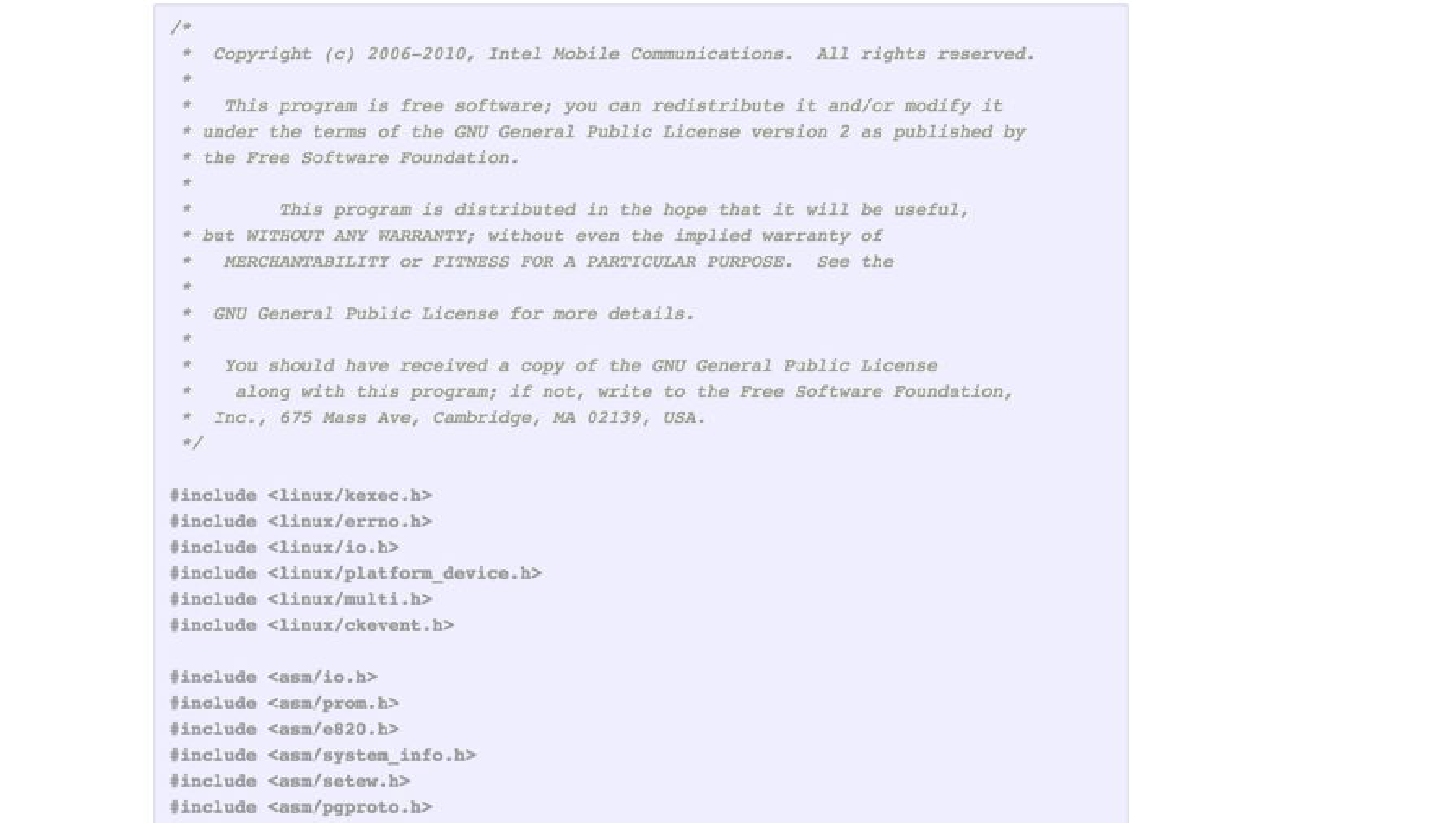
Include files, some macros, and some code.

Was this min_char_rnn ? no that is a very small toy.

There is char_rnn more mature implementation on torch, runs on GPU. - This is actually a 3 layer LSTM. 😌

Implementation Details

Torch Implementation 😌

Adventures on RNN:

Andrej and Justin pretended that they are neuroscientists. They threw a character-level RNN on some test text.

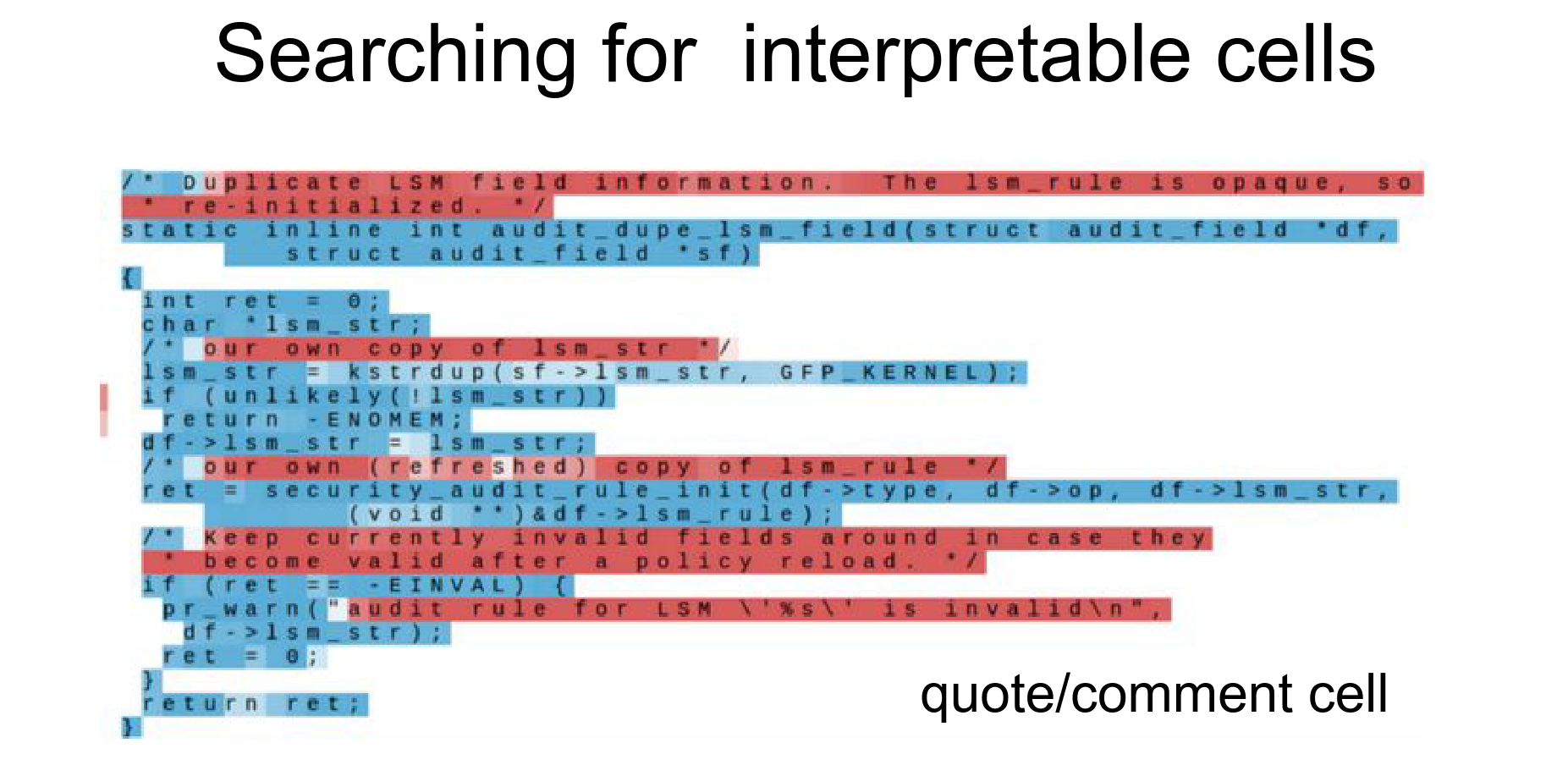
The RNN is reading the text, and as the text flows, they are looking at the hidden state of the RNN, and they are coloring the text based on whether or not that cell is excited.

Many of the hidden state neurons are not really interpretable. They fire on and off randomly.

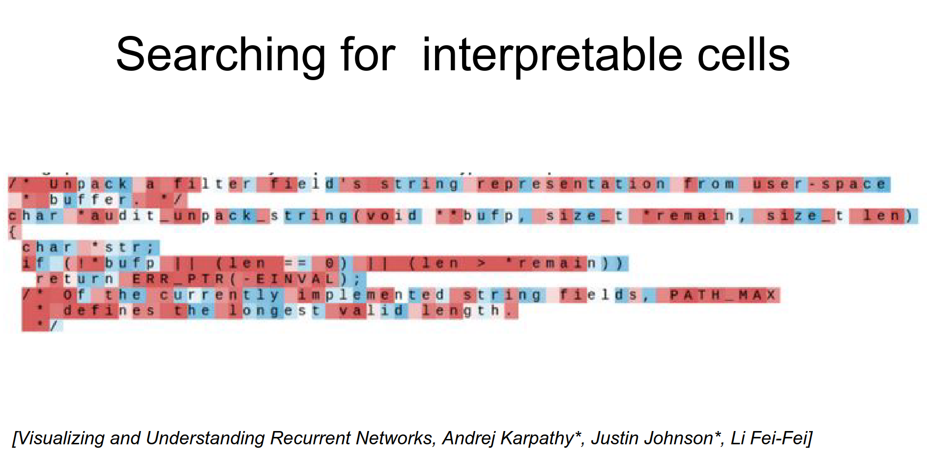
But some cells are really interpretable.

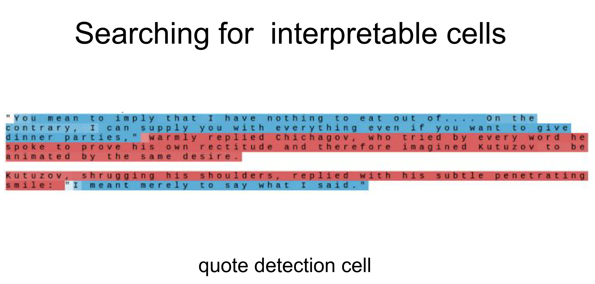
Quote Detection

It turns on when it sees a quote and it stays on until the quote closes.

The RNN decides that character-level statistics are different inside and outside of quotes. This is a useful feature to learn. So it dedicates some of its hidden state to keep track of whether or not you are inside a quote.

Sequence Length Investigation 🤔

This RNN was trained on a sequence length of 100. If you measure the length of this quote, it is much more than 100, more like 250.

We backpropagated up to 100; that is the only length that this RNN can learn itself. It would not be able to spot dependencies that are much longer than that.

But this seems to show that you can train this character-level detection cell as useful on sequences less than 100, and then it generalizes properly to longer sequences.

Generalization

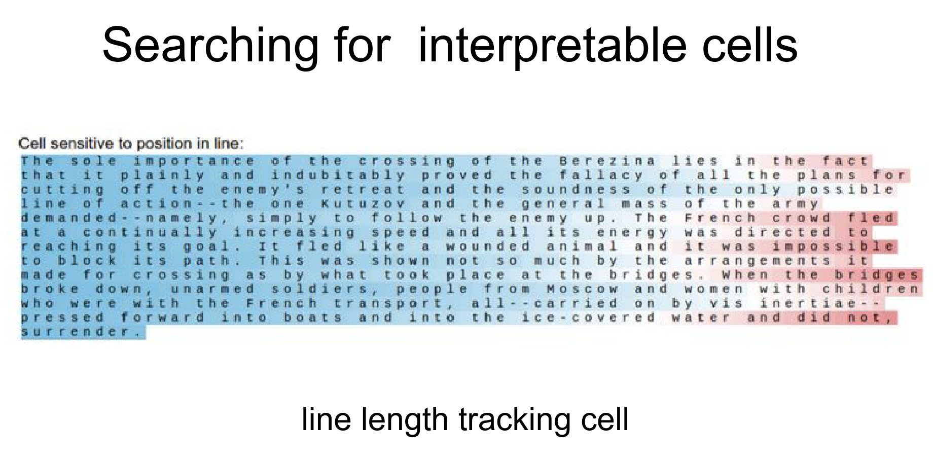
This is from War & Peace.

In this dataset, there is a \n after roughly 80 characters, every line.

There is a line length tracking cell they found; it starts at 1 and it slowly decays over time. A cell like this is really useful because this RNN needs to count 80 time steps so that it knows a newline is likely coming up next.

There are cells that only respond inside if statements.

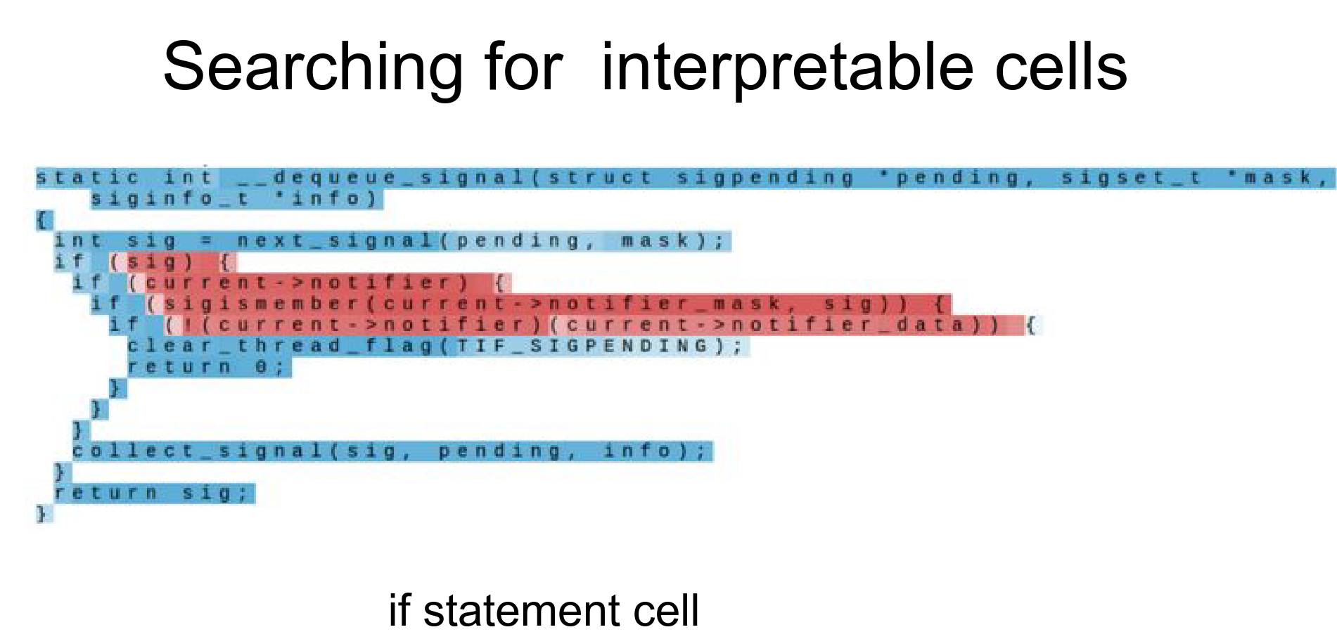
Cells that only respond inside quotes/strings.

Some cells get more excited the deeper you nest an expression.

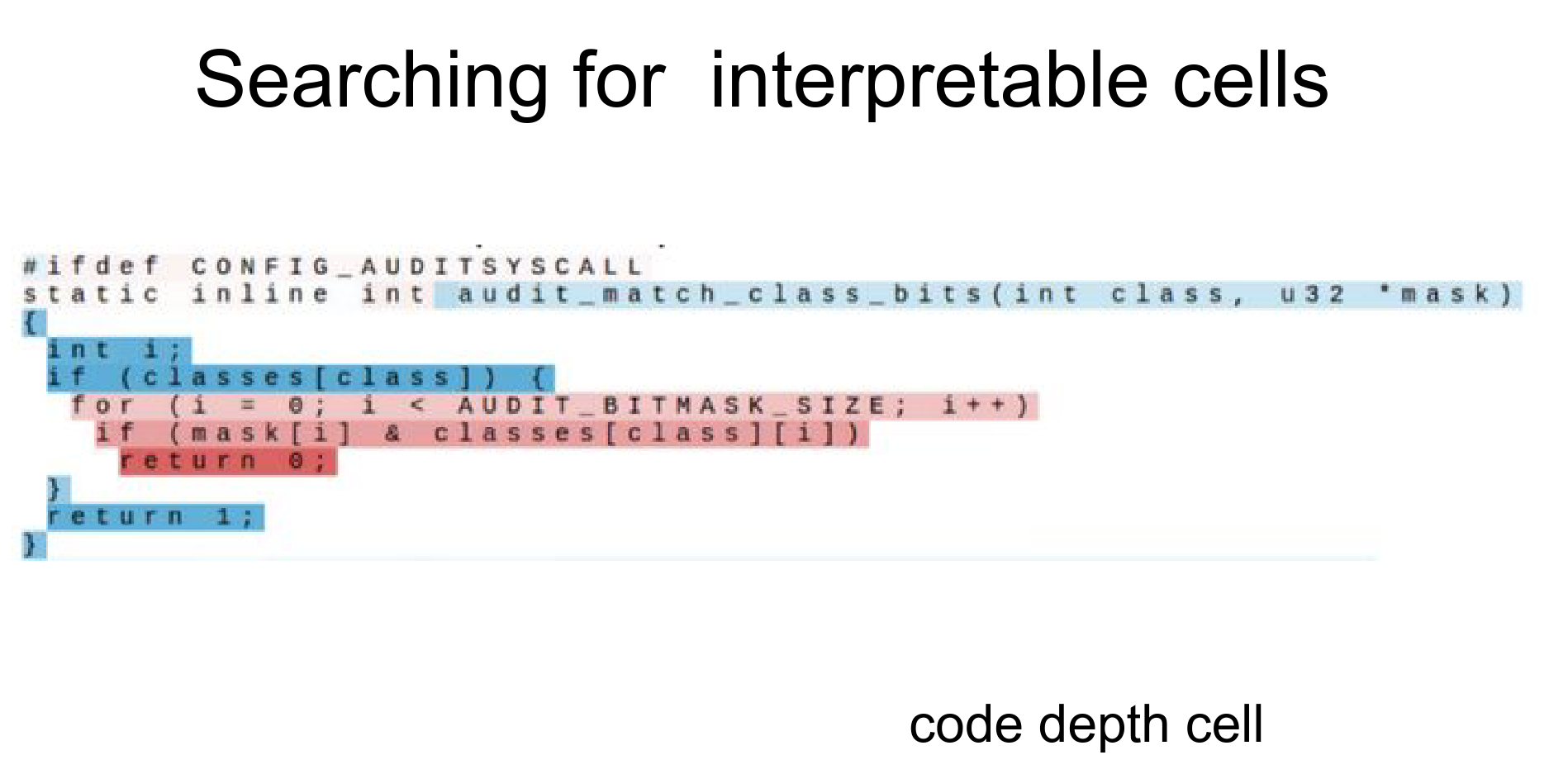
Cell Analysis

How did you figure out what individual cell is excited about?

In this LSTM you have 21,000 cells; you just kinda go through them. Manually.

Most of them look random; in 5% you spot something interesting.

We ran the entire RNN intact; we are only looking at the firing of one single cell in the RNN.

We are just recording from one cell in the hidden state, if that makes sense. I am only visualizing one part of the hidden state in the image above.

These hidden cells are always between \(-1\) and \(1\), the scale between blue and red ones.

---

RNNs in Computer Vision

Image Captioning

RNNs are pretty good at understanding how sequences form over time.

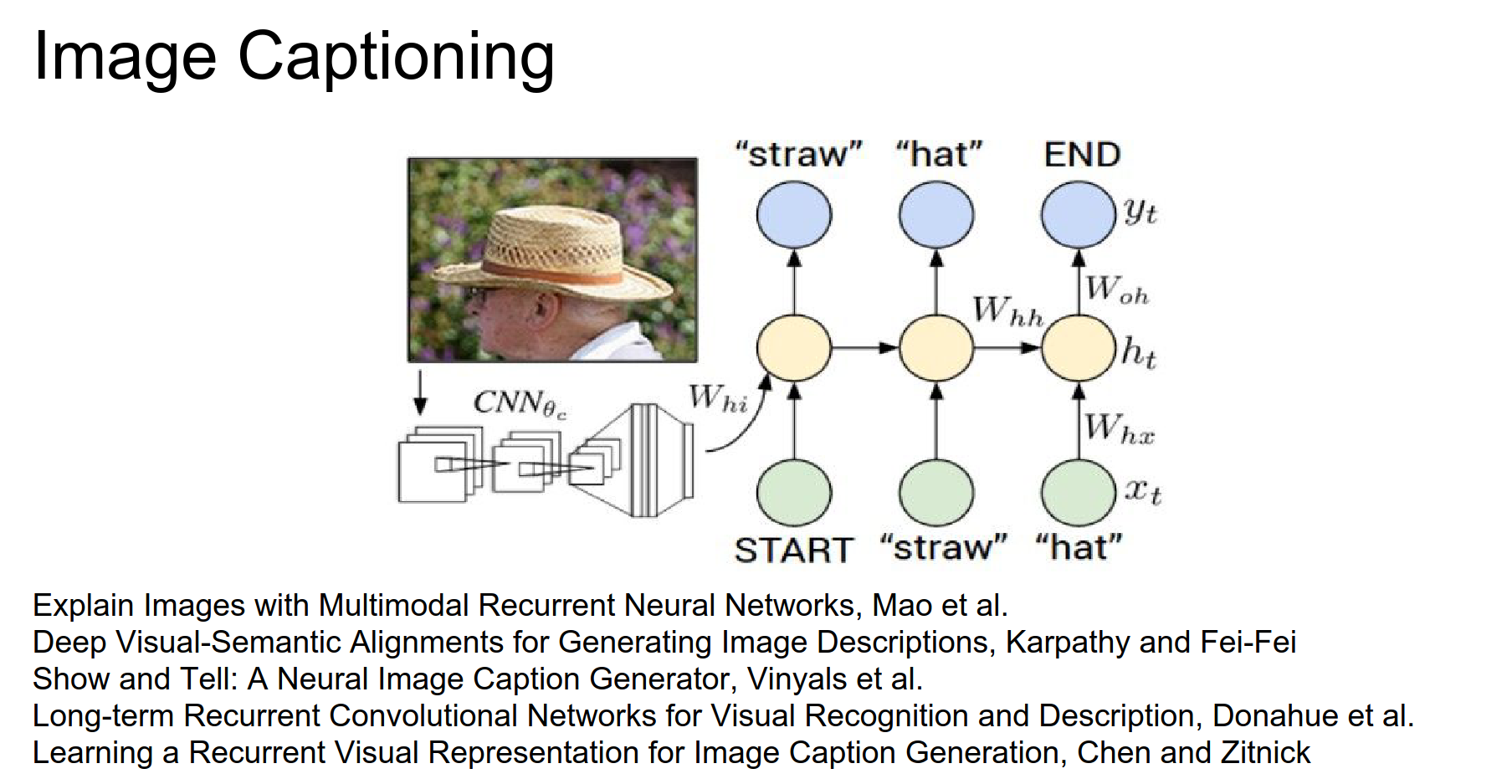
Work from 1 year ago, Andrej's paper.

Two modules: CNN processing of the image, and RNN is really good with modeling sequences.

This is just playing with Lego blocks.

We are conditioning the RNN generative model. We are not just telling it to sample text at random; we are conditioning that generative process by the output of the CNN.

This is how the forward pass happens in NN.

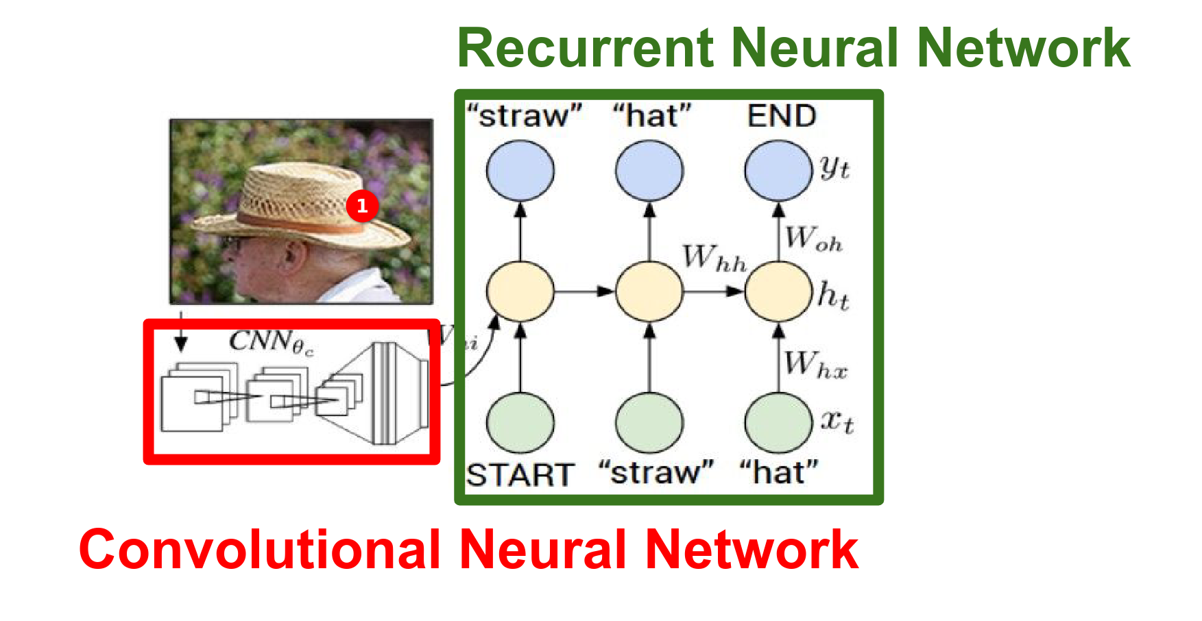
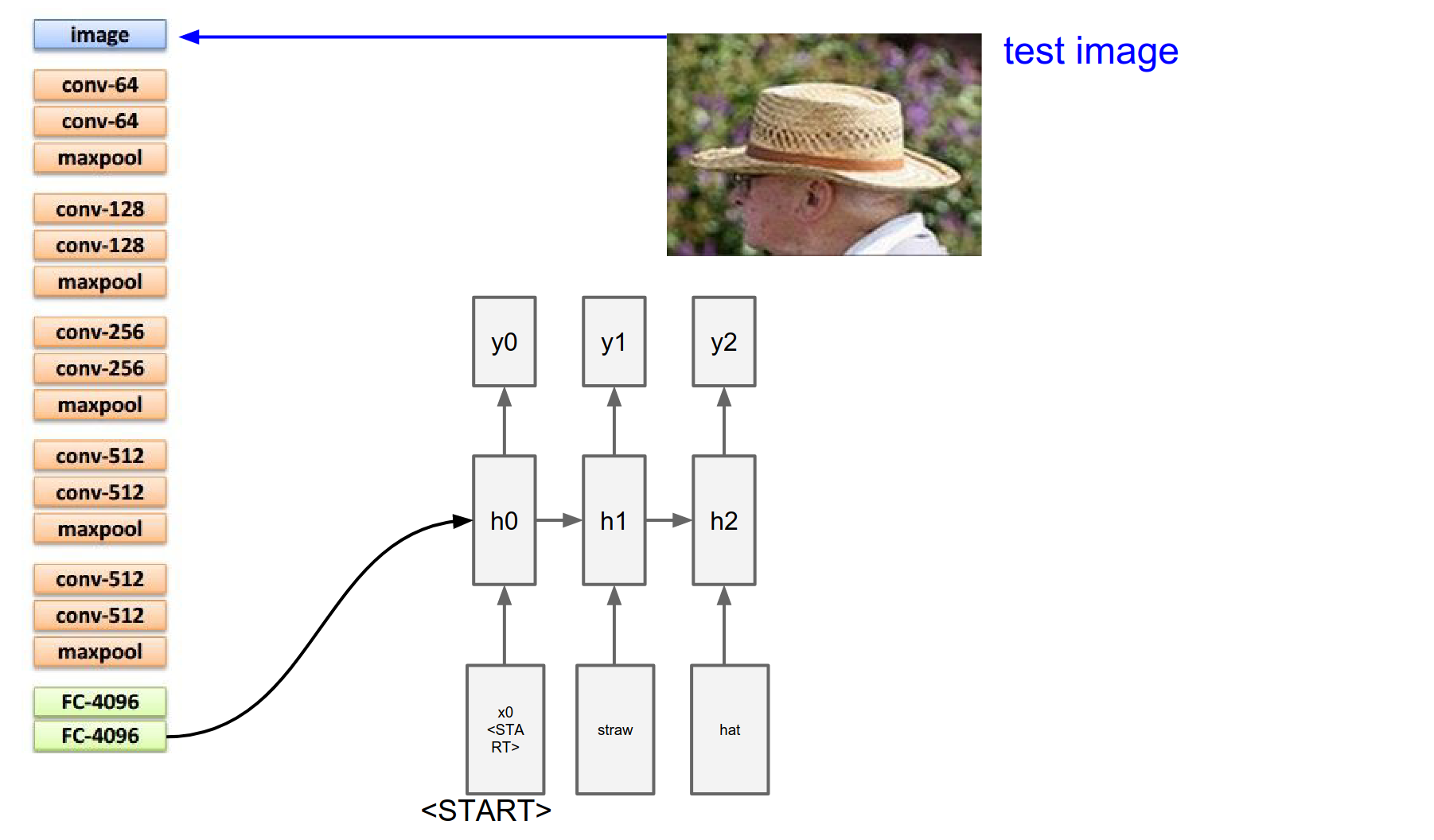
We have a test image and we are trying to describe it with a sequence of words.

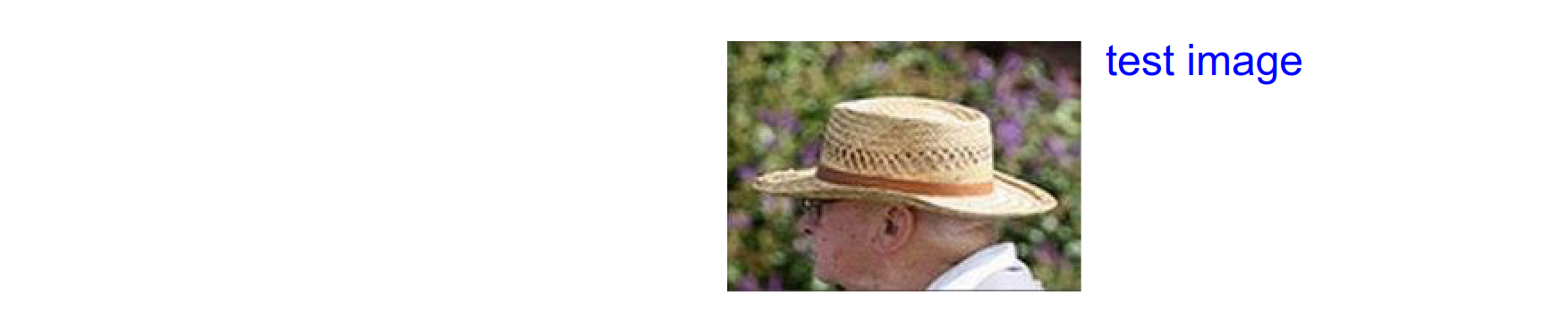
We plug it into a CNN; this is a VGGnet. We go through Conv and MaxPools until we arrive at the end.

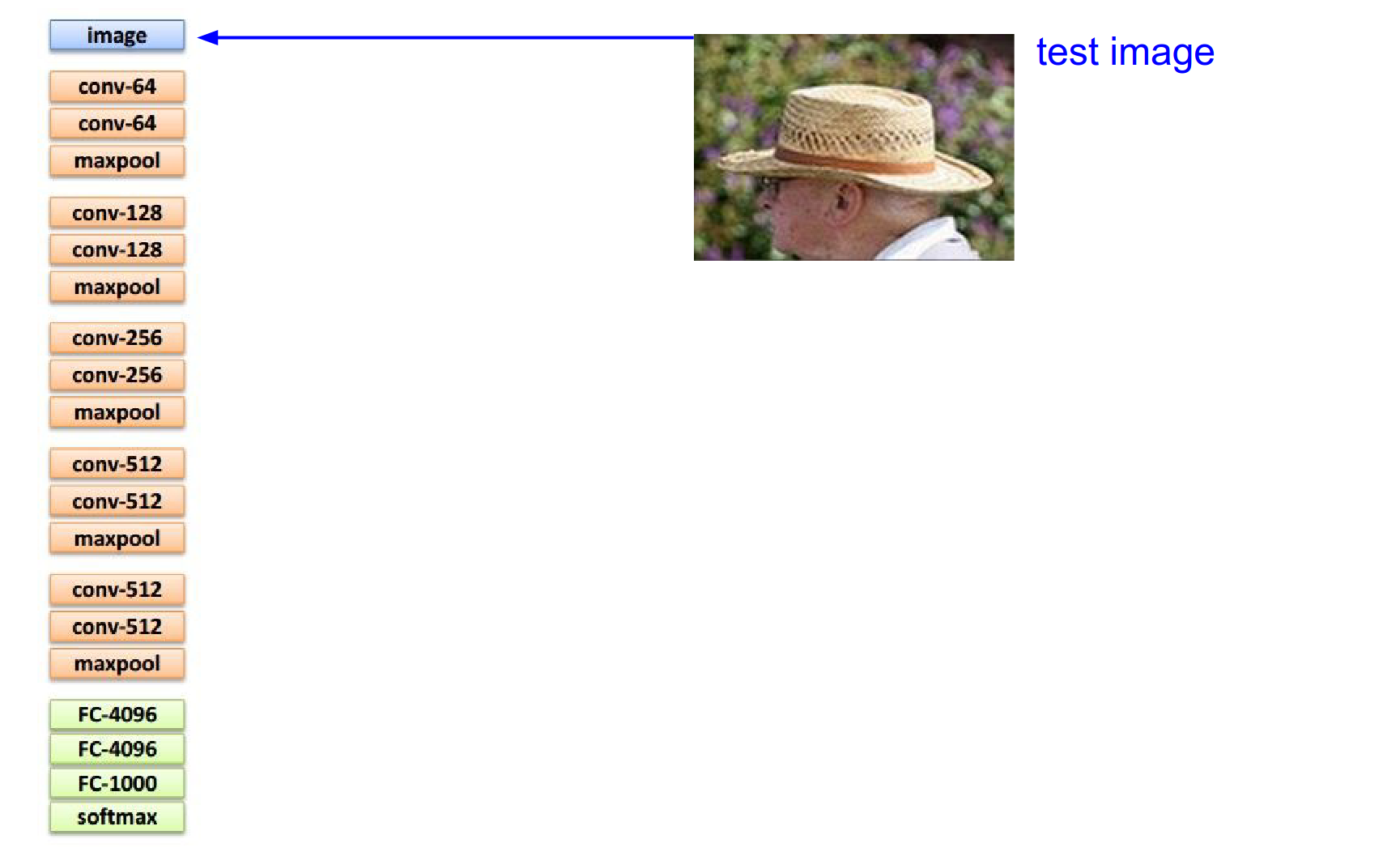
We would normally have this softmax classifier that gives us a probability distribution over 1000 classes in ImageNet. We are going to remove that classifier.

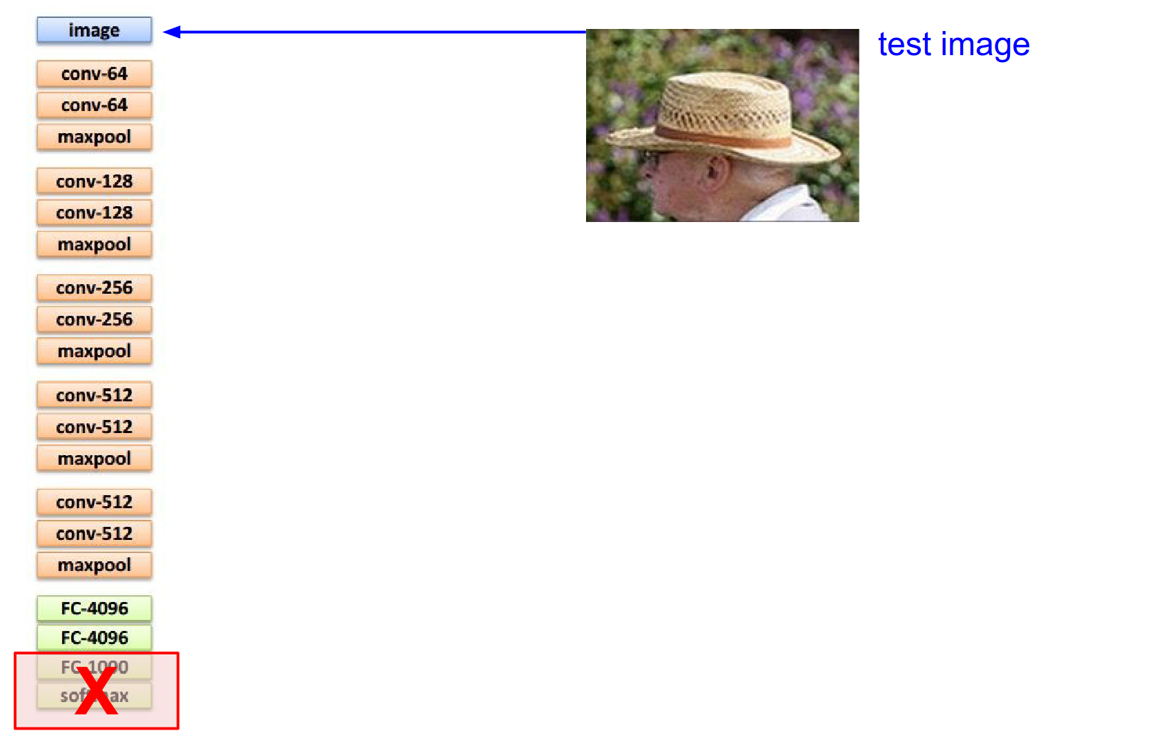
We are going to redirect the representation at the top of the network into the RNN.

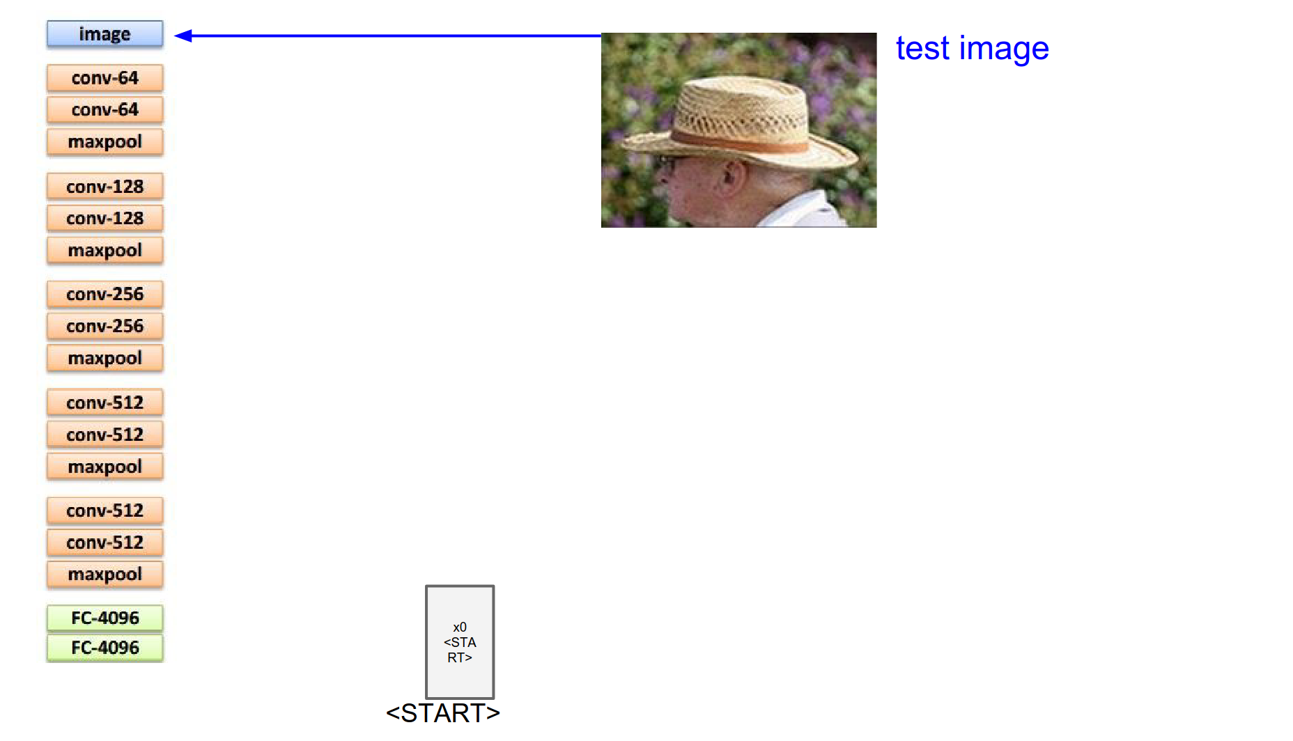
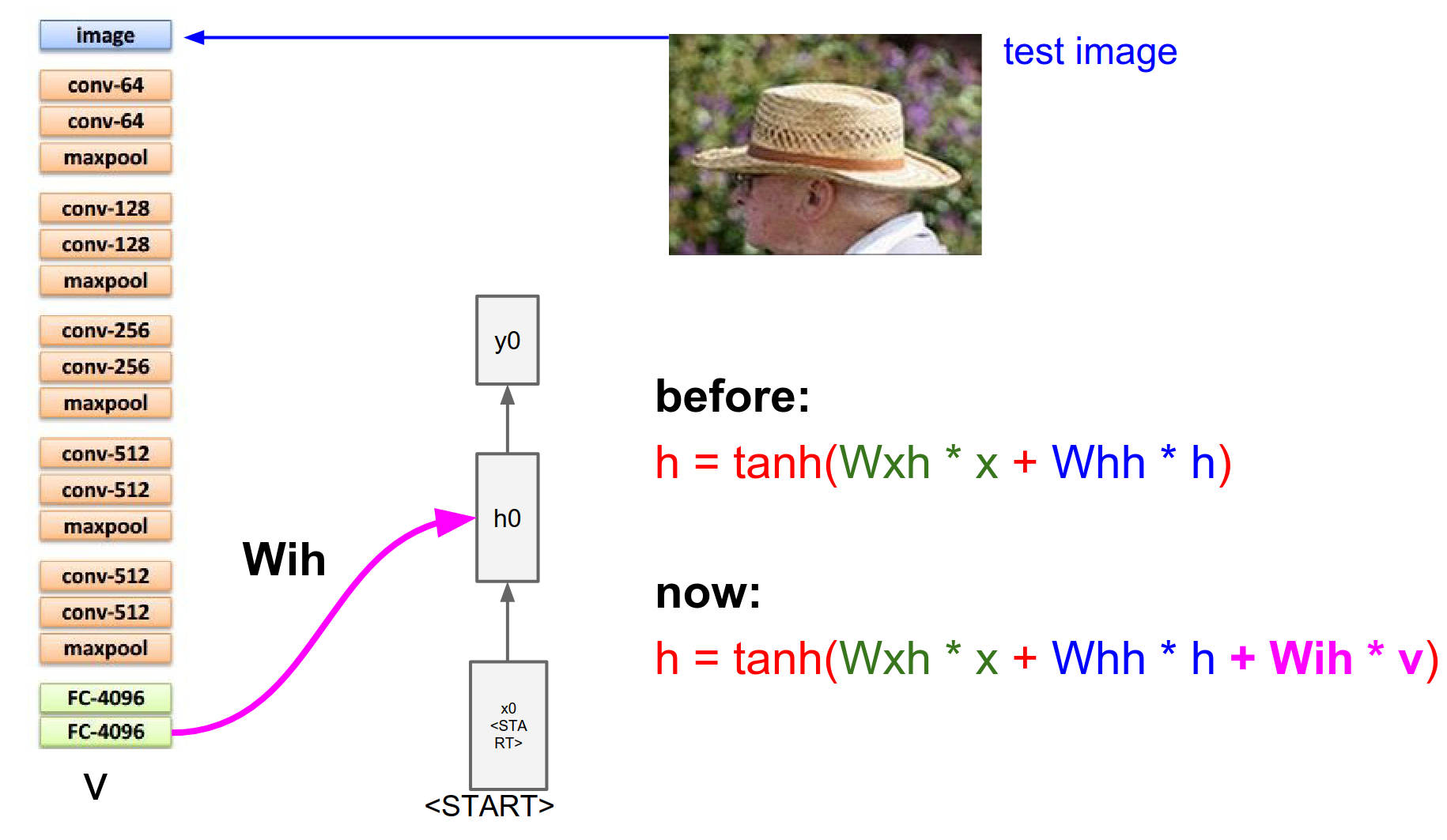
We begin with a special start vector. The input at this RNN is roughly 300-dimensional.

At the first iteration, we always use this special vector. Then we perform the recurrence formula as we saw in Vanilla RNN.

Normally we would compute the before mode. Now we are doing something different. Not only with the current input and current hidden state (which we initialized with 0 - that term goes away at the first timestep).

Image Features

This tells us how the image information is merged into the very first time step of the RNN.

There are many ways to do this plugin. This is only one of them. One of the simpler ones.

Mechanism

The straw textures can be recognized by the CNN as straw-like stuff.

Through this interaction of \(W_{ih}\), it might condition the hidden state to a particular state where the probability of the word straw can be slightly higher.

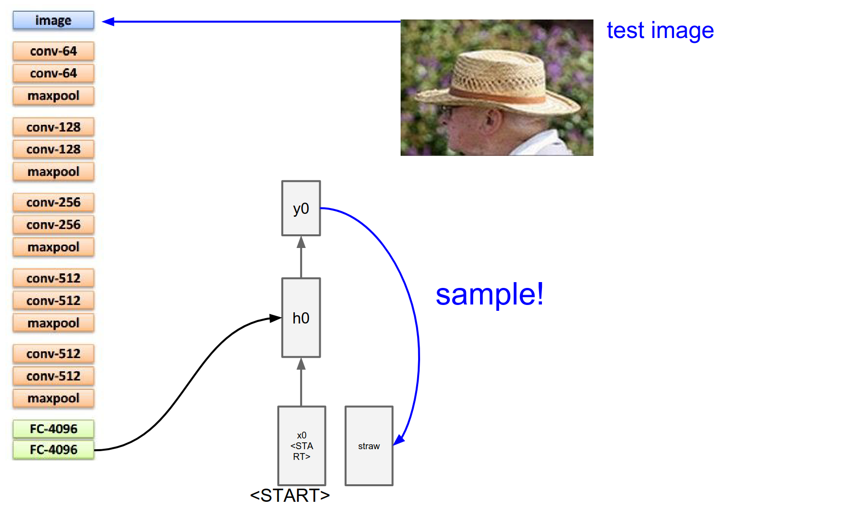
So you can imagine the textures of an image can influence the word straw, causing one of the numbers inside \(y0\) to be higher because there are straw textures in there.

RNN from now on has to juggle two tasks: it has to predict the next word in the sequence and it has to remember the image information.

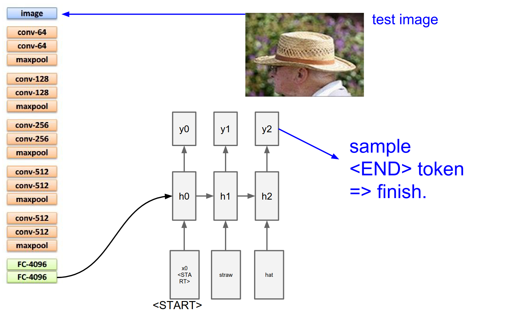
So we sample from that softmax - and suppose the most likely word that we sampled from that distribution is indeed the word straw - we would take straw and we would try to plug it into the RNN on the bottom again.

This is done by using word-level embeddings.

So the straw word is associated with a 300-dimensional vector.

Which we are going to learn by the way - we are going to learn a 300-dimensional representation for every single unique word in the vocabulary.

We plug those 300 numbers into the RNN and forward it again to get a distribution over the second word in the sequence - inside \(y1\).

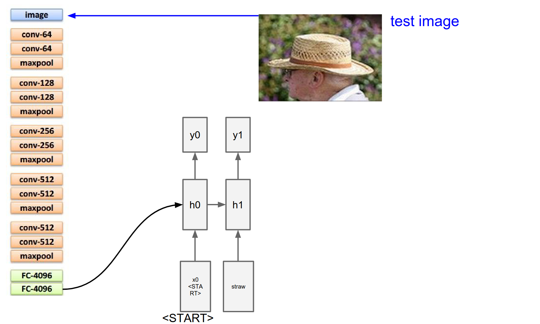
We get all these probabilities, we sample from it again.

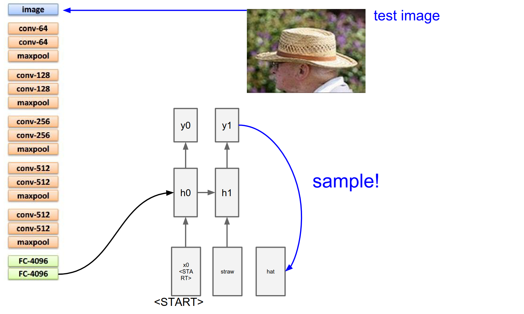
Suppose the word hat is likely now. We take the hat 300-dimensional representation vector, plug it in, and get the distribution over there.

We sample again. And we sample until we sample a special <end> token. Which is just a period at the end of the sentence.

That tells us the RNN is now done generating. The RNN has described this image as straw hat.

The number of dimensions in this \(y\) vector is number of words in your vocabulary + 1 for the special end token.

We are always feeding these 300-dimensional vectors that correspond to different words. And a special start token.

We are always backpropagating through the whole thing at a single time.

You can initialize at random, or you can initialize your VGG net pretrained from ImageNet. The RNN tells you the distributions, you encode the gradient, you backprop the whole thing as a single model.

Q&A: Embeddings

No, 300-dimensional embeddings are independent of the image. Every word has 300 numbers associated with it.

Q&A: Generative Process

We are going to backprop into it, these vectors x - so these embeddings will shift around. They are just a parameter.

It is equivalent to having a one-hot representation of all the words and a giant \(W\) matrix where we multiply \(W\) with the one-hot representation. If that \(W\) has 300 output size, it is essentially plucking out a single row of \(W\) which ends up being your embedding.

Q&A: Termination

Every training data has a special end token in it.

Q&A: Image Usage

Yes. You can plug the image at every single time step for the RNN, but that performs worse. The juggle between jobs makes it harder. It has to remember what the image has in it and it has to produce outputs.

Q&A: Data Flow

At training time, a single instance will correspond to an image and a sequence of words. We would plug the words into the RNN and we would plug that image into the CNN.

You have to be careful with different length sequences - images.

I'm willing to process batches up to 20 words and some of the sentences will be shorter and longer, and you need to (in your code) regulate that.

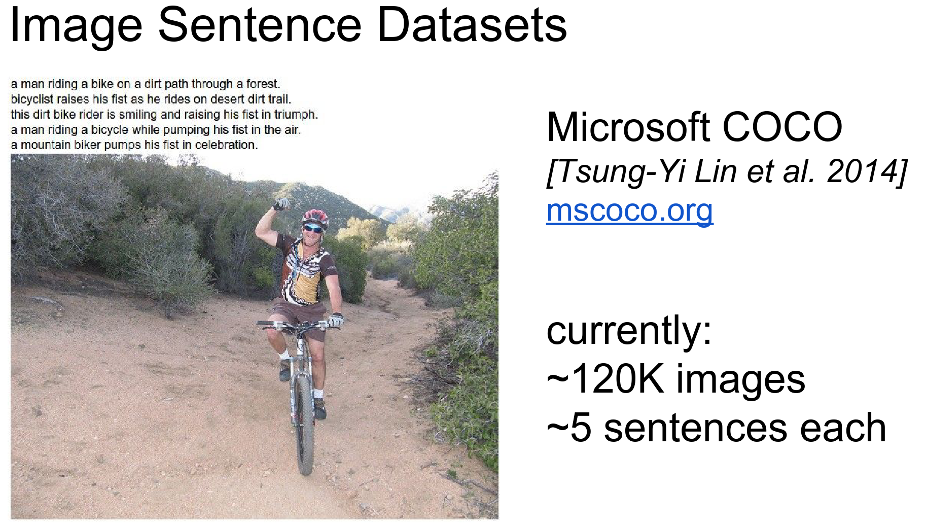
We train this Image Sentence Dataset. - MS COCO! - 120K images, 5 sentences each.

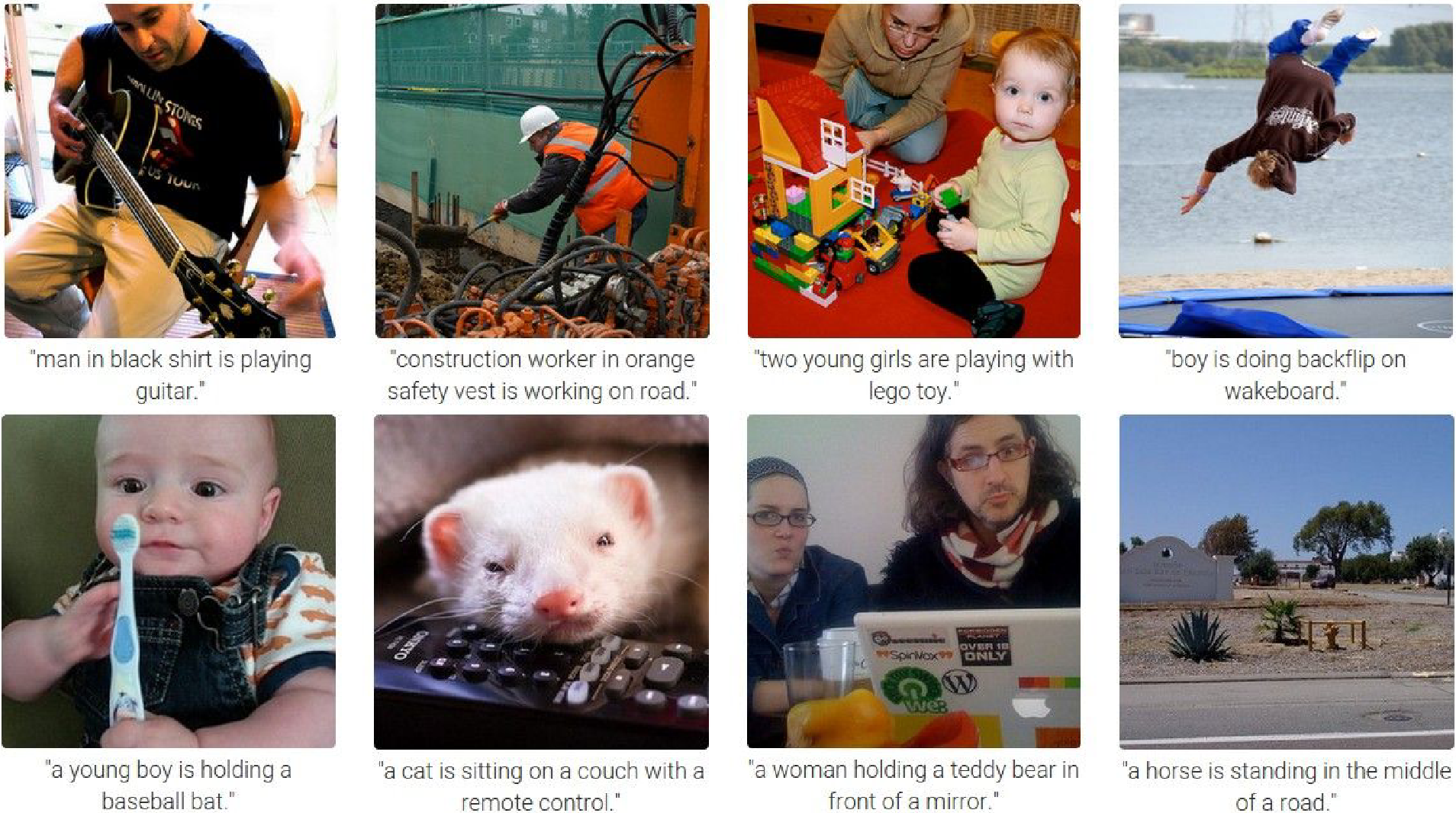
Results are down below - Boy is doing a back flip

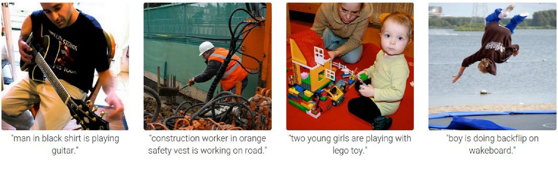
Failure cases: Cat sitting on a couch with a remote control - There is no horse.

A lot of people play with these.

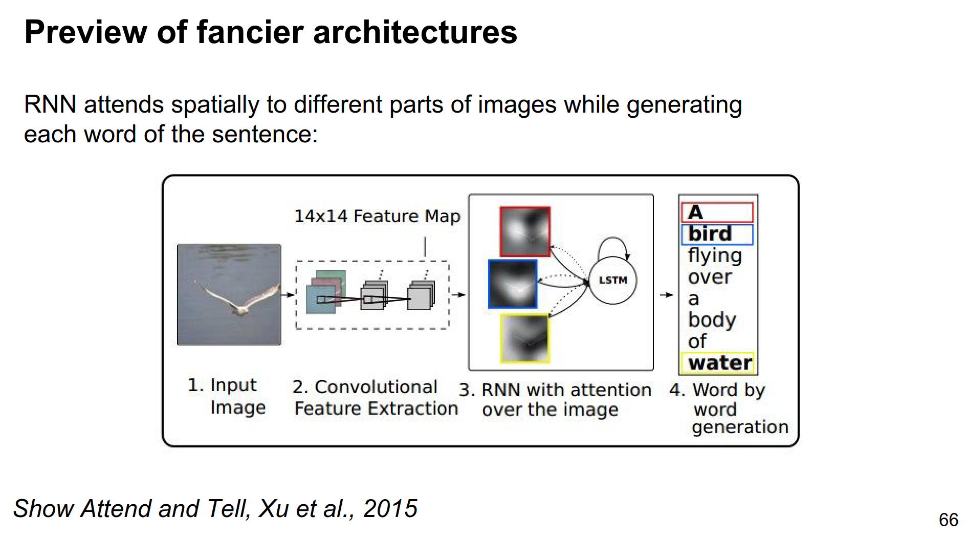
Paper from last year (2015) - Show Attend and Tell - Link.

In the current model, we only feed the image at a single time at the beginning.

Instead, you can adjust the RNN to be able to look back to the image, and reference parts of the image while it is describing the words.

As you are generating every single word, you allow the RNN to make a lookup back to the image and look for different features it might want to describe next. You can actually do this in a fully trainable way. So that the RNN not only makes the words but also decides where to look next in the image.

Attention Mechanism

The RNN not only outputs the probability distribution of the next word in a sequence, but this ConvNet gives you this volume, \(14x14x512\) activation volume, and at every single time step you do not just emit that distribution but you also emit a \(512\) distributional vector that is kinda like a lookup key.

This key is for what you want to look at next within an image.

(This implementation might not be in the paper, but this is one way you could do it.)

This key vector is emitted from the RNN; it is just predicted using some weights. This vector can be dot producted with all these \(14x14\) locations for the \(14x14x512\) activation volume.

We do all these dot products, we compute a \(14x14\) compatibility map and then we put a softmax on this, so basically we normalize this so you get what we call the attention of the image.

\(14x14\) probability map over what's interesting for the RNN, right now, over the image. Then we use this probability mask to do a weighted sum of these guys (the activation volume - \(14x14x512\)) with this saliency.

So this RNN can basically emit these vectors of what it thinks is currently interesting for it.

It goes back, and you end up doing a weighted sum of different kinds of features that the LSTM (RNN) wants to look at at this point in time.

Example

As the RNN generates, it might decide like: okay, I'd like to look for something object-like now

It emits a vector of 512 numbers of object-like stuff. It interacts with the ConvNet activation volume, and maybe some of the object-like regions of that volume light up.

And the saliency map, in the \(14x14\) array, ends up focusing your attention on that part of the image through this interaction.

Image Lookups

Soft Attention

We will go into this. RNN can have selective attention over its inputs as it's processing the inputs.

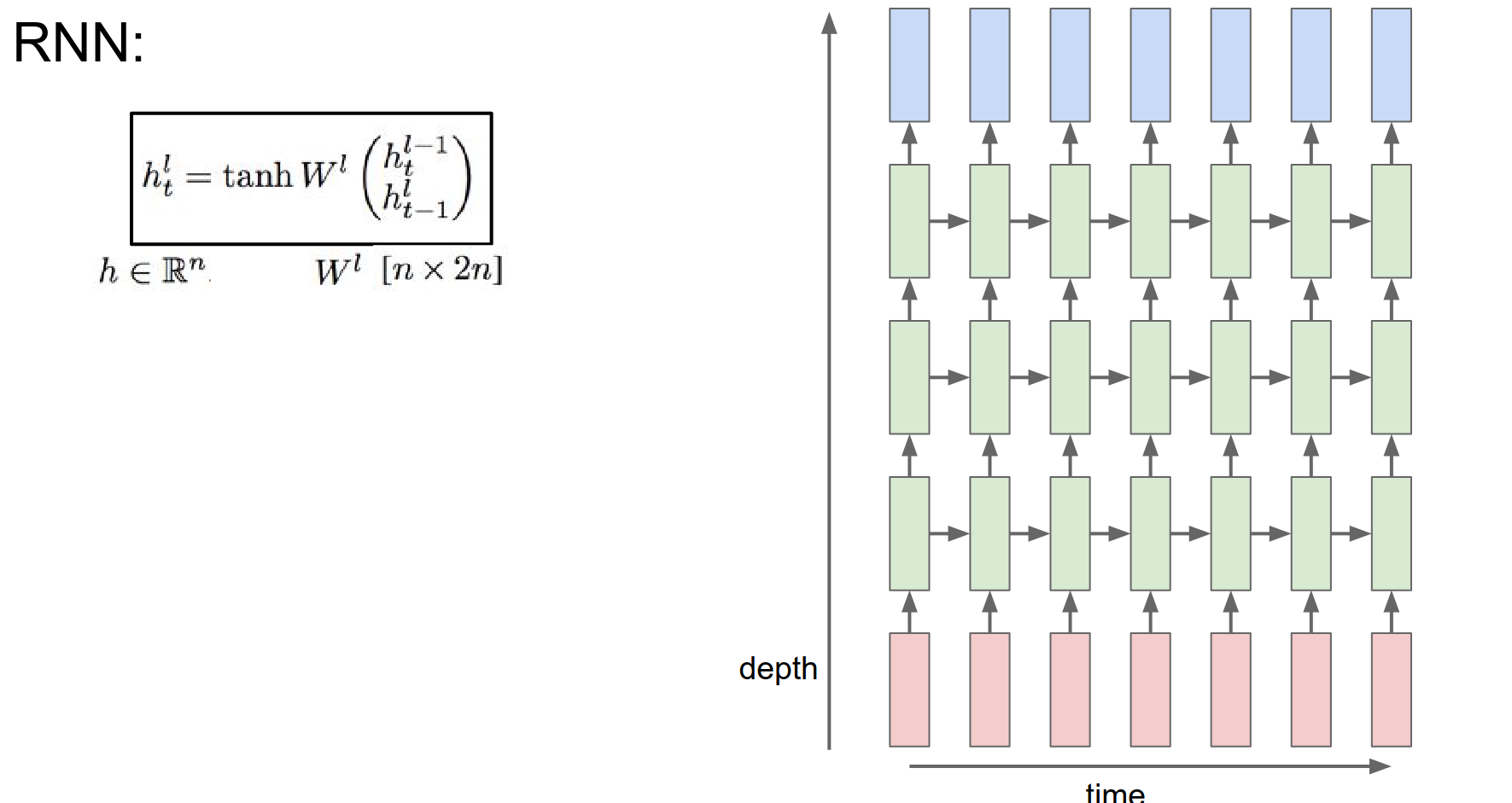
If we want to make RNNs more complex, we can stack them up in layers.

More deep stuff usually works better.

There are many ways to do this. One way is to straight up plug RNNs into each other.

The input for one RNN is the hidden state vector of the previous RNN.

In the image below, we have time on the horizontal axis and different RNNs on the vertical.

3 separate RNNs. Each with their own set of weights. These RNNs just feed into each other. This is trained jointly. Single computational graph we backpropagate through.

We are still doing the exact same thing as we were doing before. Using the same formula.

We are taking a vector from below in depth and before in time, we are concatenating them and we are putting them through this \(W^l\) transformation, and squish them with a \(tanh()\).

What we had before:

\[h = tanh(W_{xh} * x + W_{hh} * h)\]

You can rewrite this as a concatenation of \(x\) and \(h\) multiplied by a single matrix.

As if you stacked x and h into a single vector.

\[\begin{bmatrix} x \\ h \\ \end{bmatrix}\]

Then I have this \(W\):

\[\begin{bmatrix} W_{hx} & W_{xx} \end{bmatrix} \]

We can use this to have a single \(W\) transformation.

These RNNs are now indexed by both time and layer in which they occur.

Another way to stack them is to use a better recurrence formula.

In practice, you will rarely use a formula like this. This is very rarely used.

Instead, you will use:

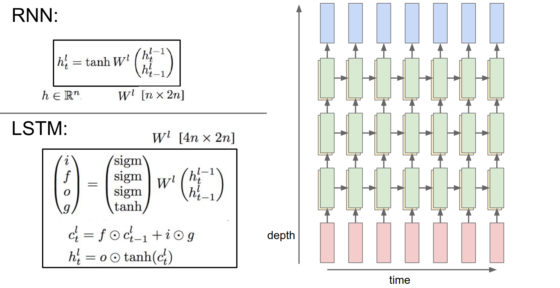
LSTM

This is used in all the papers now.

Everything is exactly the same as within RNN, it's just that the recurrence formula is a slightly more complex function.

We are still taking the hidden vector from below in depth, like your input, and before in time, previous hidden state. We are concatenating them, putting them through a \(W\) transform.

But now we have this new complexity on how we achieve the new hidden state at this point in time.

We are just being slightly more complex in how we combine the vector from below and below to perform the update of the hidden state.

LSTM vs RNN

Why are we using sigmoids and tanh() together??

These diagrams are not helping anyone. They really scared Andrej the first time he saw them.

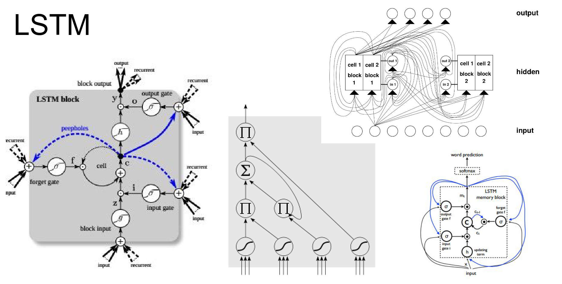
LSTM is tricky to put in a diagram, so let's go over it step by step.

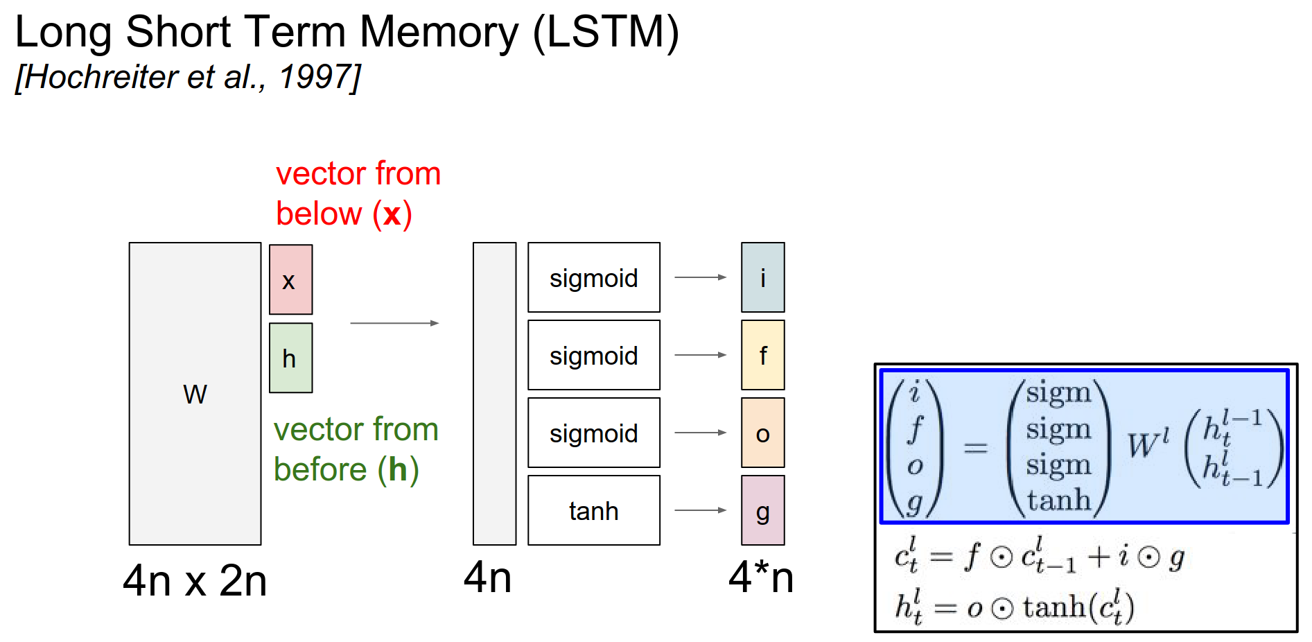
x is input, h is previous hidden state, we mapped them through the transformation \(W\), and if both \(x\) and \(h\) are of size \(n\) - there are \(n\) numbers in them - we are going to end up producing \(4n\) numbers.

We have 4 dimensional vectors, \(i\), \(f\), \(o\) and \(g\) (they are short for input, output, forget, and g).

The \(i\), \(f\), \(o\) go through sigmoid gates. The \(g\) goes through tanh gate.

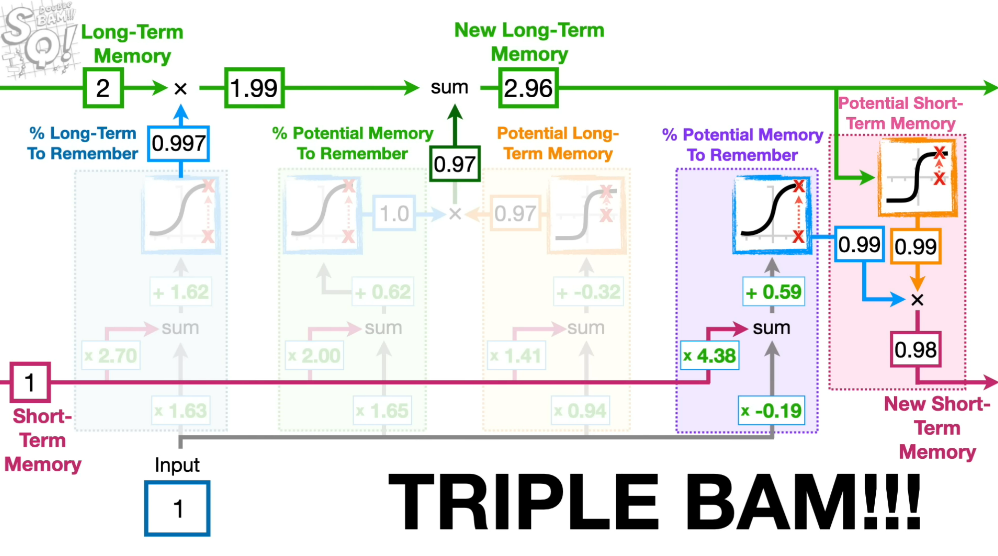
Normally an RNN only has a single vector \(h\) at every single time step. LSTM has 2 vectors at every single time step, the hidden vector \(h\) and the cell state vector \(c\).

Above in the image, we have green \(h\) vectors and yellow \(c\) vectors for LSTM.

LSTMs are operating this cell state, so depending on what's before you and below you (that is your context) you end up operating on the cell state with these \(i\), \(f\), \(o\) and \(g\) elements.

Think of \(i\), \(f\), \(o\) as binary, either 0 or 1 (we are computing them based on our context). We of course gate them with sigmoids because we want to backpropagate over them, we want them to be differentiable.

The \(c\) formula is, based on what the gates are, and what \(g\) is, we are going to update this \(c\) value.

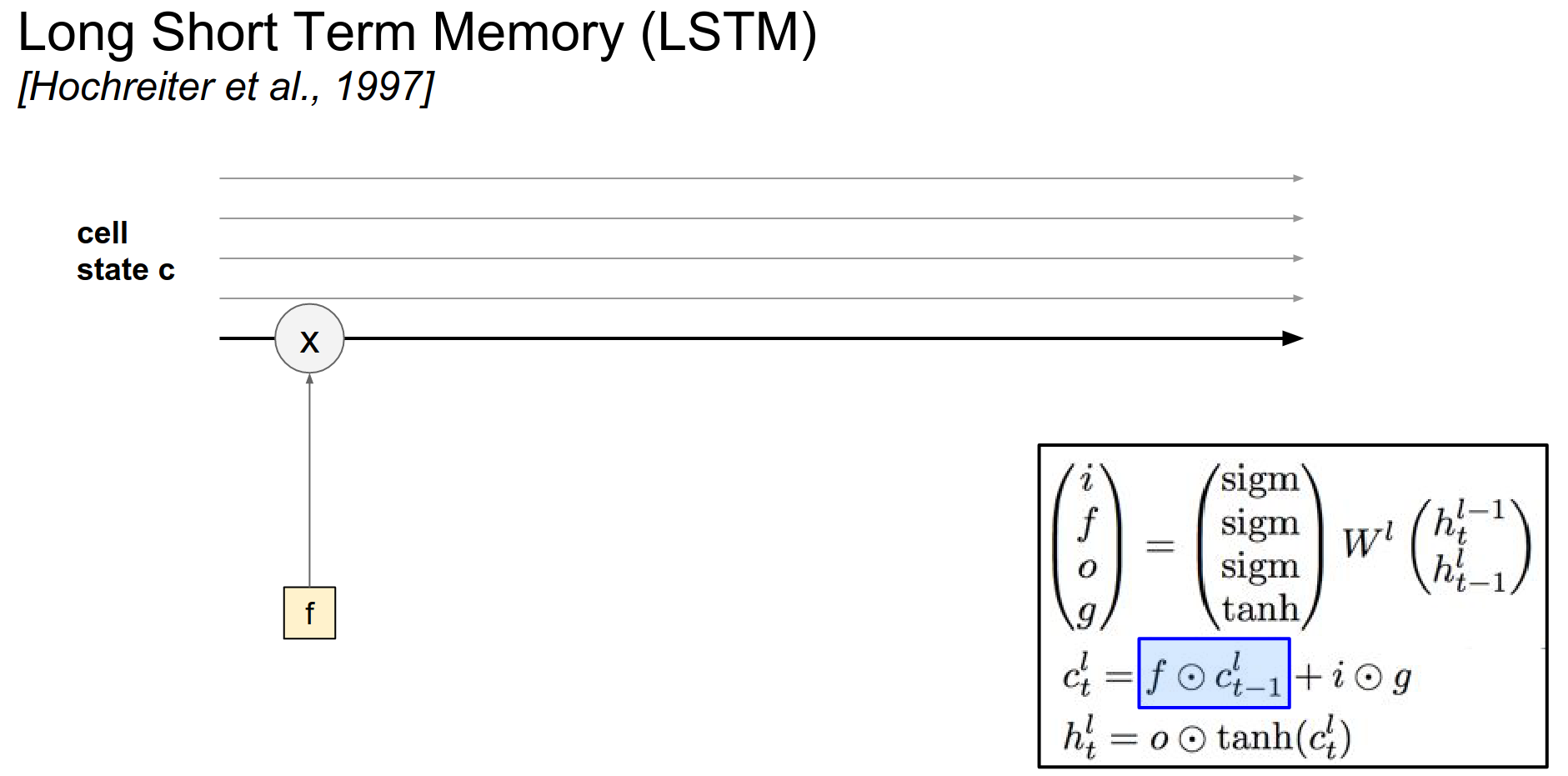
In particular, the \(f\) is called the ==forget== gate, that will be used to reset some of the cells to zero.

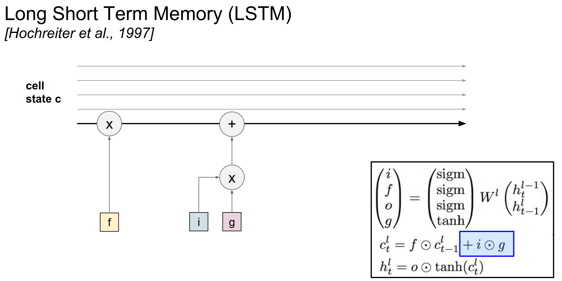
The cells are best thought of as counters. These counters, we can either reset them to zero with the \(f\) interaction (\(f . c_{t-1}\)). Or we can also add to a counter, through the interaction of \(i.g\).

Since \(i\) is between 0 and 1 and \(g\) is between -1 and 1, we are basically adding a number between -1 and 1 to every cell.

At every single time step we have these counters, and all the cells. We can reset the counters to 0 with a forget gate or we can choose to add a number between -1 and 1 to every single cell.

Cell Update

The hidden update ends up being a squashed cell - \(tanh(c)\) that is modulated with this output gate \(o\).

Hidden State Leakage

We only chose to reveal some of the cells to the hidden state in a learnable way.

---

We are adding a number between -1 and 1 with \(i.g\) here. That might be confusing, because if we only had a \(g\) there instead, \(g\) is already between -1 and 1.

Gate Rationale

If you think about \(g\), it is a linear function of your context squashed by \(tanh()\).

If we were adding just \(g\) instead of \(i.g\), that would be a really simple function, so by adding the \(i\) in there having a multiplicative interaction, you are going to end up having a richer function that you can express.

Express in terms of what we are adding to our cell state as previous \(h\)'s.

Another way to think about this, we are decoupling these two concepts of: - how much do we want to add to a cell state (which is \(g\)) - do we want to add to a cell state (which is \(i\))

\(i\) is do we actually want this operation to go through, and \(g\) is what do we want to add.

By decoupling these 2, that also dynamically has some nice properties in terms of how this LSTM trains.

Cell Flow

Think about this as cells going through, the first interaction is \(f . c\).

\(f\) is an output of a sigmoid. So \(f\) is basically gating your cells with a multiplicative interaction. -> If \(f\) is 0, you will shut off the cell and reset the counter.

This \(i.g\) part is basically adding to the cell state.

And then the cell state leaks into the hidden state, but it only leaks through a tanh(). And that gets gated by \(o\).

The \(o\) vector can decide which parts of the cell state to actually reveal to the hidden cell.

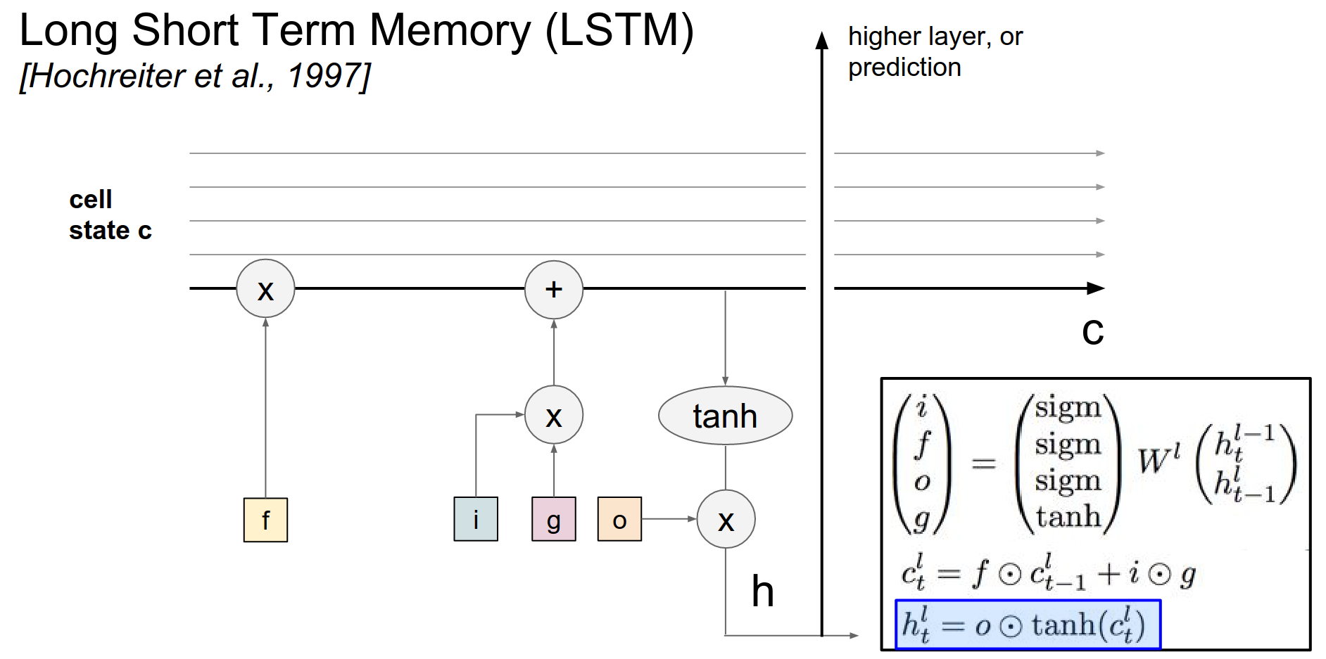
Then you will notice that this hidden state not only goes to the next iteration of the LSTM, but it also flows up to higher layers ->

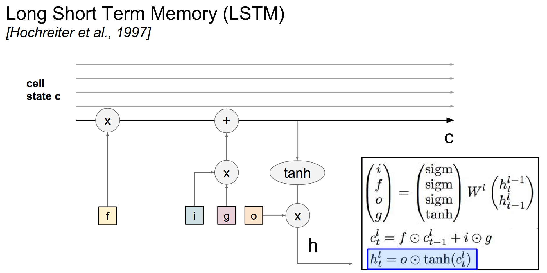
Because this is the hidden state vector we end up plugging into further LSTMs above us. Or that goes into a prediction.

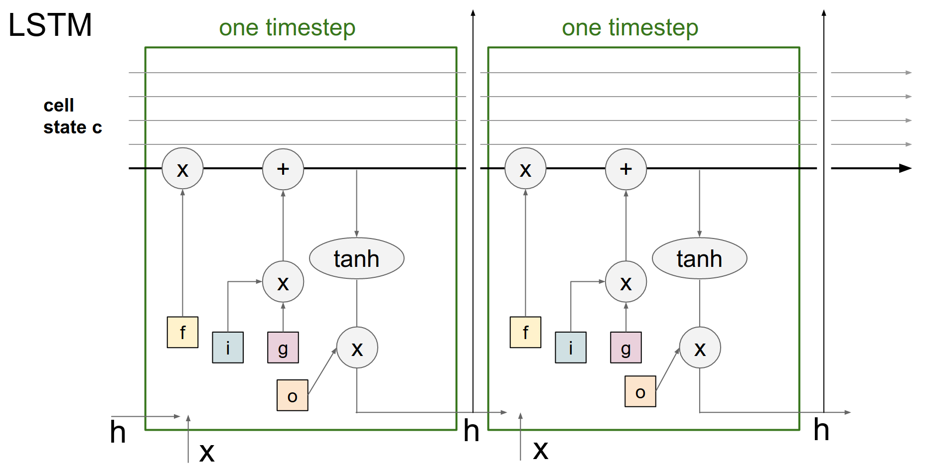
When you unroll this, basically the way it looks like is kinda like down below.

Diagram 😅

LSTM Summary 😍

You get your input vectors from below, your hidden state from before.

The \(x\) and \(h\) determine your gates, \(i\), \(f\), \(g\) and \(o\) -> they are all n dimensional vectors.

They end up modulating how you operate over the cell state.

This cell state can, once you actually reset some counters and once you add numbers between -1 and +1 to your counters, the cell state leaks out (some of it) in a learnable way, then it can either go up to the prediction or it can go to the next iteration of the LSTM going forward.

Motivation 🤔

There are many variances to an LSTM, people play a lot with these equations (the hidden state and the cell state), we have converged on this (what we explained) as being the reasonable thing. There are many little tweaks that you can make that do not deteriorate your performance by a lot.

You can remove some of the gates.

The \(tanh()\) of \(c\) can be just a single \(c\), that will work fine. \(tanh()\) will make it work slightly better.

It actually kinda makes sense, in terms of, just these counters can be reset to zero or you can add small numbers between -1 and 1 to them.

Advantages 🤔

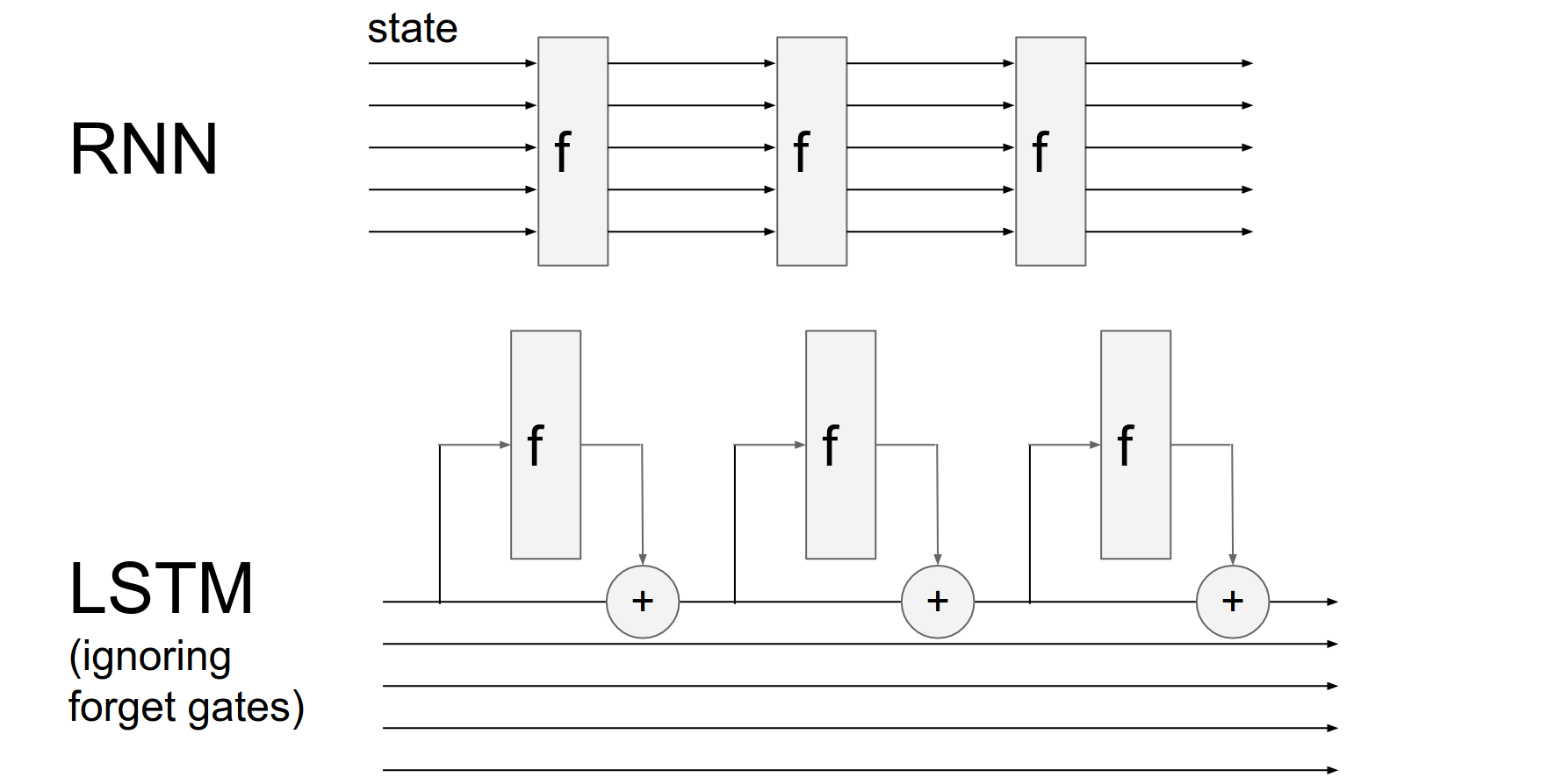
RNN has some state vector. You are operating over it, and you are completely transforming it through this recurrence formula.

So you end up changing your hidden state formula from time step to time step.

LSTM instead has these cell states flowing through, we are looking at the cells, some of it leaks into the hidden state, based on the hidden state we are deciding how to operate over the hidden cell.

And if you ignore the forget gates then we end up with basically just tweaking the cell by additive interaction.

There is some stuff that is a function of the cell state, then whatever it is we end up, additively changing the cell state, instead of just transforming it right away.

It's an additive instead of transformative interaction.

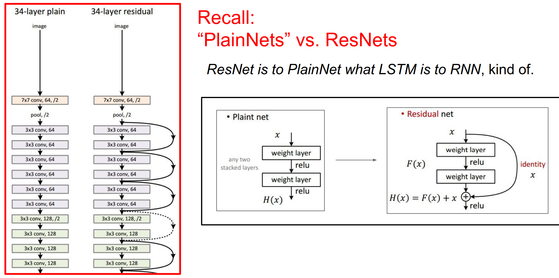
ResNet Connection

Normally with a ConvNet we are transforming the representation, ResNets has these skip connections, so ResNets has these additive interactions, so we have this \(x\) (identity in the image down below), we do some computation based on \(x\), then we have an additive interaction with \(x\).

ResNet Block

We have these additive interactions, where \(x\) is basically your cell, and we go off and we do some function and we choose to add to this cell state.

But LSTMs unlike ResNets have these forget gates, these forget gates can choose to shut off some parts of the signal. Otherwise it very much looks like a ResNet.

We are converging into like very similar looking architectures that work in ConvNets and in RNNs where it seems like dynamically it is much nicer to have these additive interactions that allow you to backpropagate much more effectively.

Backpropagation Dynamics 🤔

In the LSTM, if we inject some gradients signal at some time steps here, if we inject some gradient signal at the end of the diagram, then these plus interactions (in the image above) are just like a gradient super highway.

These gradients will flow through all the addition interactions, because addition distributes gradients equally.

So if we plug in any gradient at any point in time here it is just going to flow all the way back.

And of course the gradient also flows through these \(f\)'s and they end up contributing their own gradients into the gradient flow, but you will never end up with what we referred to with RNN's problem called vanishing gradients.

Vanishing Gradients - RNN vs LSTM

Where these gradients just die off - go to zero - as we backpropagate through. In RNN we have this vanishing gradient problem, in LSTM because of this super highway of additions, these gradients at every single time step that we inject into the LSTMs from above, just flow through to cells. Your gradients do not end up vanishing.

---

Extra image, magenta line in bottom is hidden state, green line at top is cell state.

---

Why do RNNs have terrible backward flow?? 😮

In the link we are unrolling an RNN in many time steps. We are injecting gradient at \(128\) time step. And we are backpropagating the gradients through the network. And we are looking at what is the gradient for input to hidden matrix, at every single time step.

In order to get the full update through the batch, we end up adding all these gradients here.

So we made this injection and we are back propping through time. The image is just showing the slices of that backpropagation.

There is just a grey image in the RNN, LSTM is kinda like all random.

The LSTM will give you a lot of gradients through this backpropagation. A lot of information that is flowing through.

In the RNN it just dies off, gradient vanishes. Just becomes tiny numbers.

In kinda like 8-10 time steps, all the gradient information that we injected, did not flow through the network. So you cannot learn very long dependencies because of all the correlation structure has been just dying down.

---

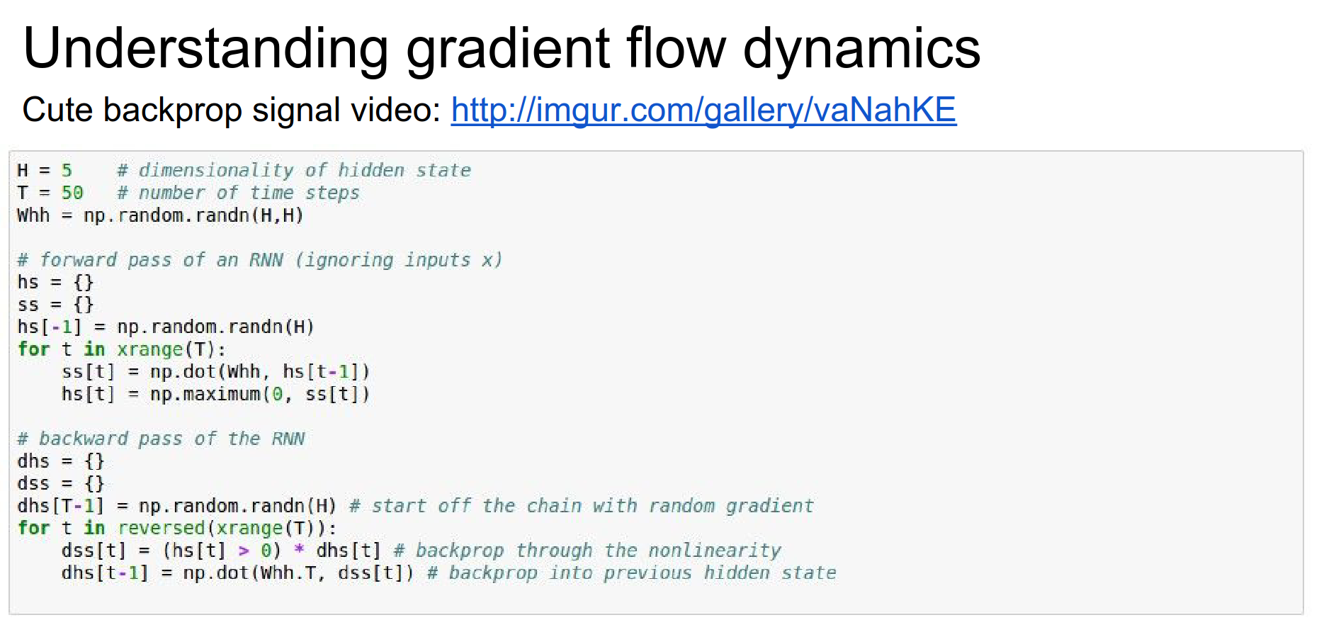
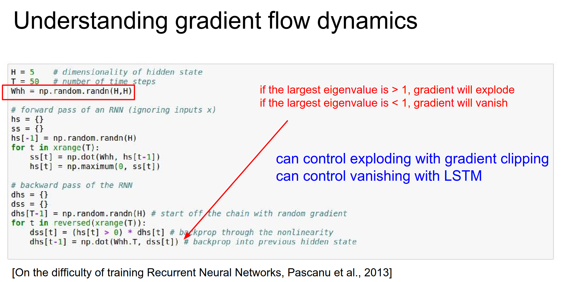
We have an RNN here that Andrej will unroll.

Not showing inputs, we only have hidden state updates.

whh is hidden to hidden interaction. We will basically forward this Vanilla RNN for some t timesteps.

whh times previous time step hs[t-1] and ReLU on top of that -> np.maximum()

This was the forward pass, ignoring the inputs.

In the backward pass, injecting a random gradient at the last time step. Then we will go backwards and backpropagate. When we backprop this we have to backprop through a ReLU, we need to backprop through a Whh multiply, and ReLu again and Whh multiply and so on.

In the for loop down below (for t in reversed(xrange(T))), we are just thresholding anything where the inputs were less than zero. And we are back propping the Whh * h operation.

Something funky going on when you look at what is happening to this dhs which is the gradient on the h's, as you go backwards through time, it has a funny structure that is worrying. As you look at how this gets chained up in the loop.

What are we doing with these time steps? What is not good? 🤔

We are multiplying by this Whh matrix over and over and over again.

When we backprop through all the hidden states, we end up backpropagating this Whh * hs, the backprop turns out to be that, you take your gradients signal and then you multiply by the Whh matrix.

So we end up with 50 times multiplication with Whh - thresholded ...

You can think of this as two scalars. You have a random number 1 and you keep multiplying with number 2, over and over and over again. What happens?

If number 2 is not \(1\), the number either dies - 0 - or explodes.

Here we have matrices not numbers, but the same thing happens.

If the spectral radius of this Whh matrix - which is the largest eigenvalue of that matrix - if it is greater than one, then this gradient will explode. If it is lower than 1, the gradients will die.

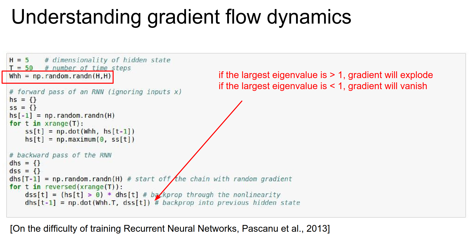
Terrible dynamics. In practice, you can control the exploding gradient - one simple hack is to clip it.

Really patchy solution - gradient clipping 🤭

When they vanish, GG in RNN. LSTM is really good for vanishing gradients, because of these highways of cells which are only changed with additive interactions where the gradients just flow, they never die down.

We always use LSTMs and we do gradient clipping, because the gradients can explode still.

Do not forget, these super highways are only true when we do not have any forget gates (because they can just make gradients 0). People play with that bias in forget gate sometimes.

---

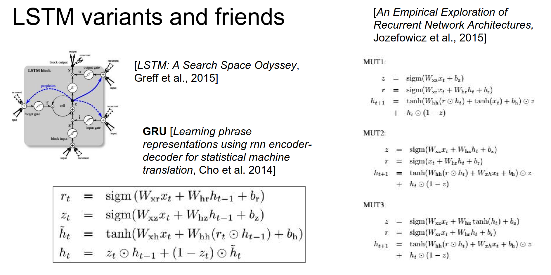
They tried really different things on LSTM.

"LSTM: A Search Space Odyssey" by Greff et al. presents a comprehensive analysis of various Long Short-Term Memory (LSTM) variants and their impact on the performance of recurrent neural networks (RNNs).

What they do:

• The authors evaluate eight different LSTM variants, each with a single modification to the standard LSTM architecture.
• They test these LSTM variants on three representative tasks: speech recognition, handwriting recognition, and polyphonic music modeling.
• To ensure a fair comparison, the authors use random search to select the hyperparameters for each dataset and LSTM variant, resulting in a total of 5,400 trials.

Why they do it:

• LSTMs have become the state-of-the-art models for many machine learning problems, but there is a lack of systematic studies on the utility of the different computational components within the LSTM architecture.

• The authors aim to fill this gap by isolating the impact of each LSTM component and understanding its contribution to the overall performance of the model.

What they achieve:

• The study provides valuable insights into the effectiveness of various LSTM components, such as the forget gate, input gate, and output gate, among others.
• The results show that some LSTM variants perform better than the standard LSTM architecture on certain tasks, suggesting that the optimal LSTM configuration may depend on the specific problem and dataset.
• The authors also discuss the historical evolution of the LSTM architecture, highlighting the importance of understanding the role of each component in the model's performance.

In summary, the "LSTM: A Search Space Odyssey" paper conducts a comprehensive analysis of LSTM variants, aiming to shed light on the utility of different computational components within the LSTM architecture. The findings contribute to a deeper understanding of LSTM models and can guide future research and development in the field of recurrent neural networks.

---

There is this thing called GRU? Paper 💖

It is a change on an LSTM, also has these additive interactions, but what is nice about it is it has a shorter smaller formula. And it only has a single \(h\) vector. Implementation wise this is nicer - in forward pass.

Smaller, simpler that seems to have the benefits of an LSTM, it almost always works equally with LSTM.

Raw RNN does not work really well. LSTMs and GRUs are used. They have these additive interactions which allow solving the vanishing gradient problem.

We gotta do gradient clipping.

We need better understanding.

Done with lecture 10.