12. Overview of Caffe/Torch/Theano/TensorFlow

Part of CS231n Winter 2016

---

Lecture 12: Deep Learning Libraries

Today we're going to go over the four major software packages that people commonly use for deep learning: Caffe, Torch, Theano, and TensorFlow.

The final assignment is due on Wednesday.

---

A quick note: if you're using terminal instances for your projects, make sure you are backing up your code and data. We've had some problems where instances crash, and while data is usually recoverable, it can take time.

---

Framework Overview

Disclaimer: I've mostly worked with Caffe and Torch, so I know the most about them. I'll do my best to give you a good flavor for the others as well.

Caffe

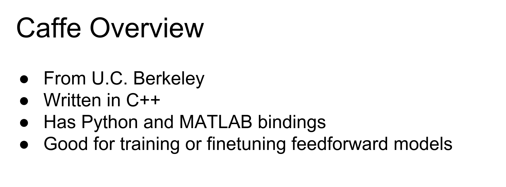
Caffe sprung out of a paper at Berkeley that tried to re-implement AlexNet and use AlexNet features for other things. Since then, Caffe has grown into a really popular, widely used package, especially for Convolutional Neural Networks.

Caffe is mostly written in C++. There are bindings for Python and MATLAB that are super useful.

In general, Caffe is really widely used and is great if you just want to train standard feed-forward vanilla Convolutional Networks.

Caffe is somewhat different from the other frameworks in that you can actually train big powerful models without writing any code yourself. For example, you can train a ResNet ImageNet classification model using Caffe without writing any code, which is pretty amazing.

The most important tip when working with Caffe is that the documentation is sometimes out of date. Be courageous, dive in and read the source code yourself.

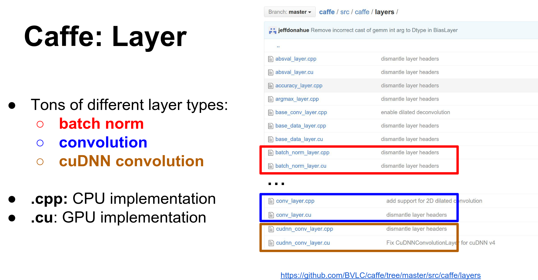
The C++ code in Caffe is pretty well-structured and easy to understand. If you have doubts about how things work, your best bet is to go on GitHub and read the source code.

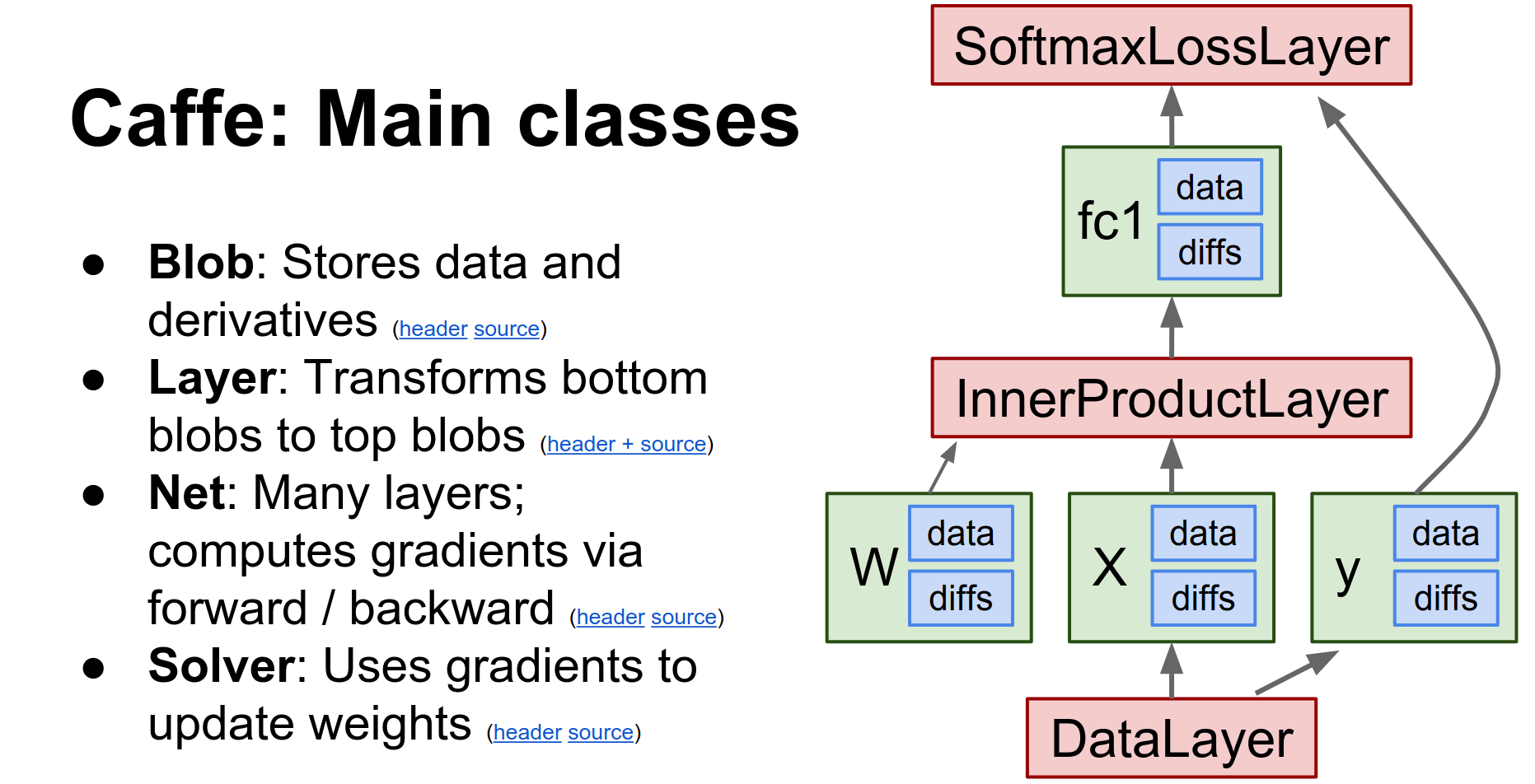
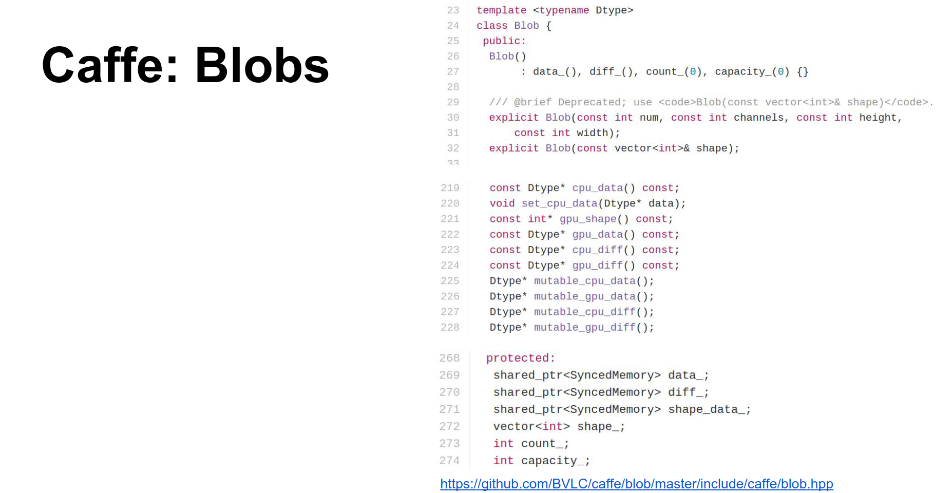
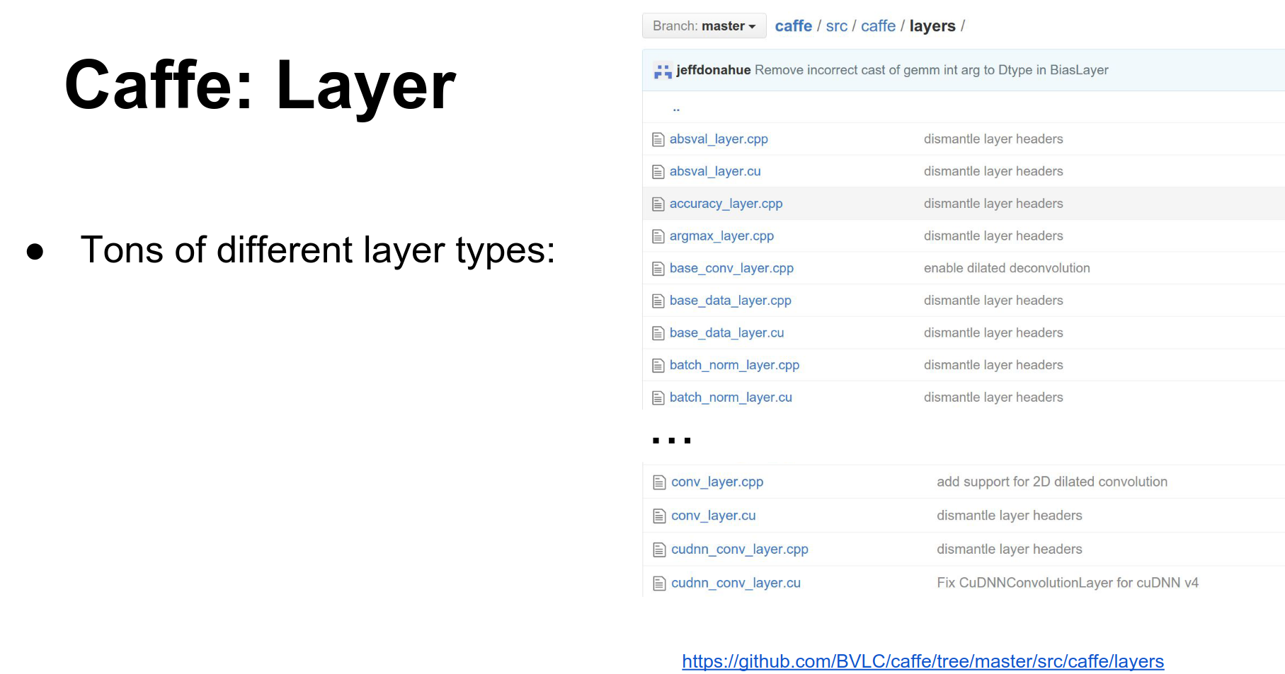
Caffe is a huge project, but there are really four major classes you need to know about:

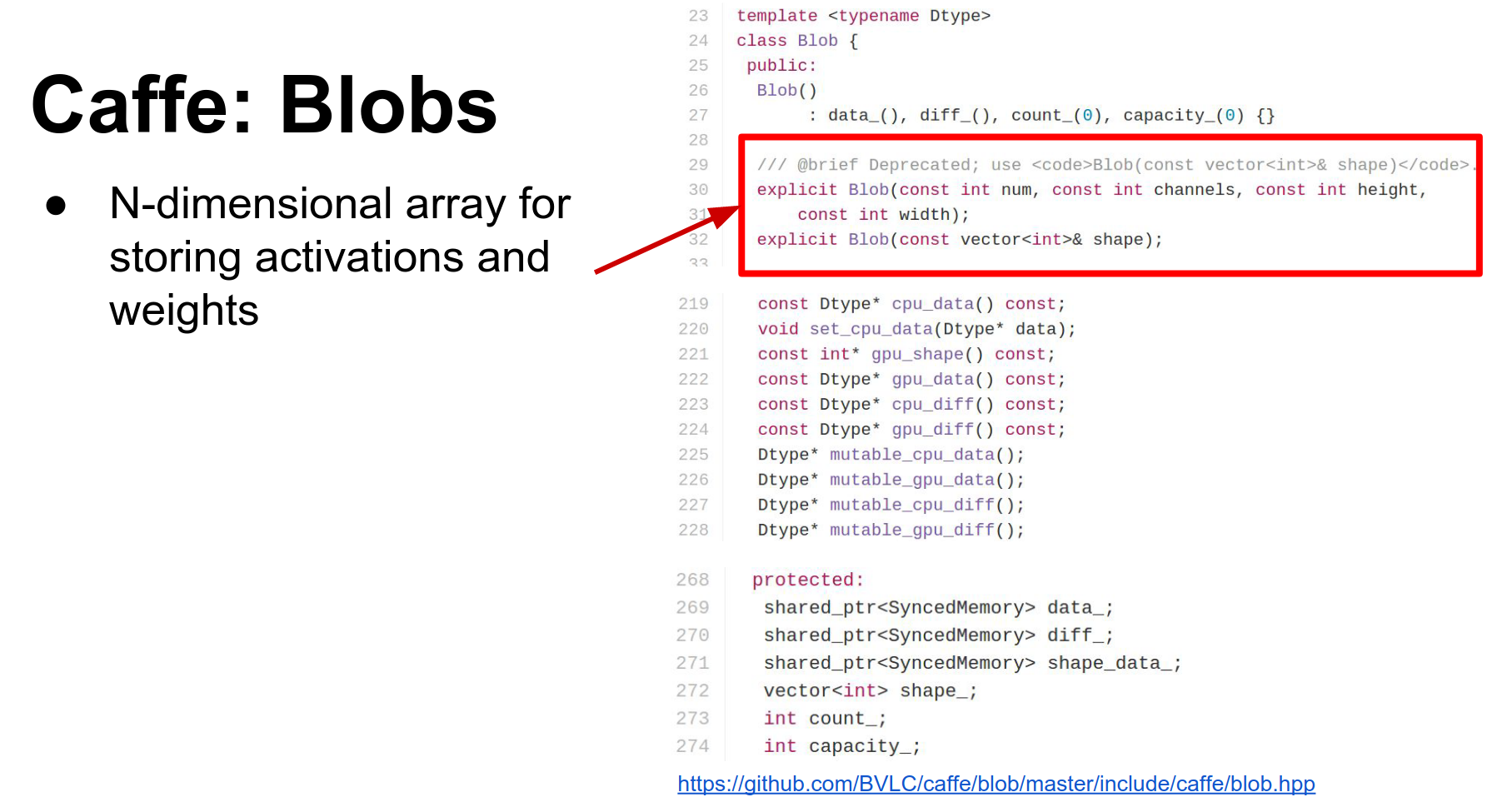
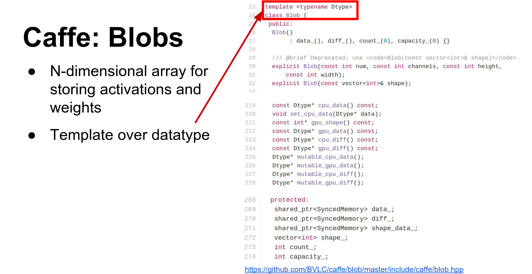
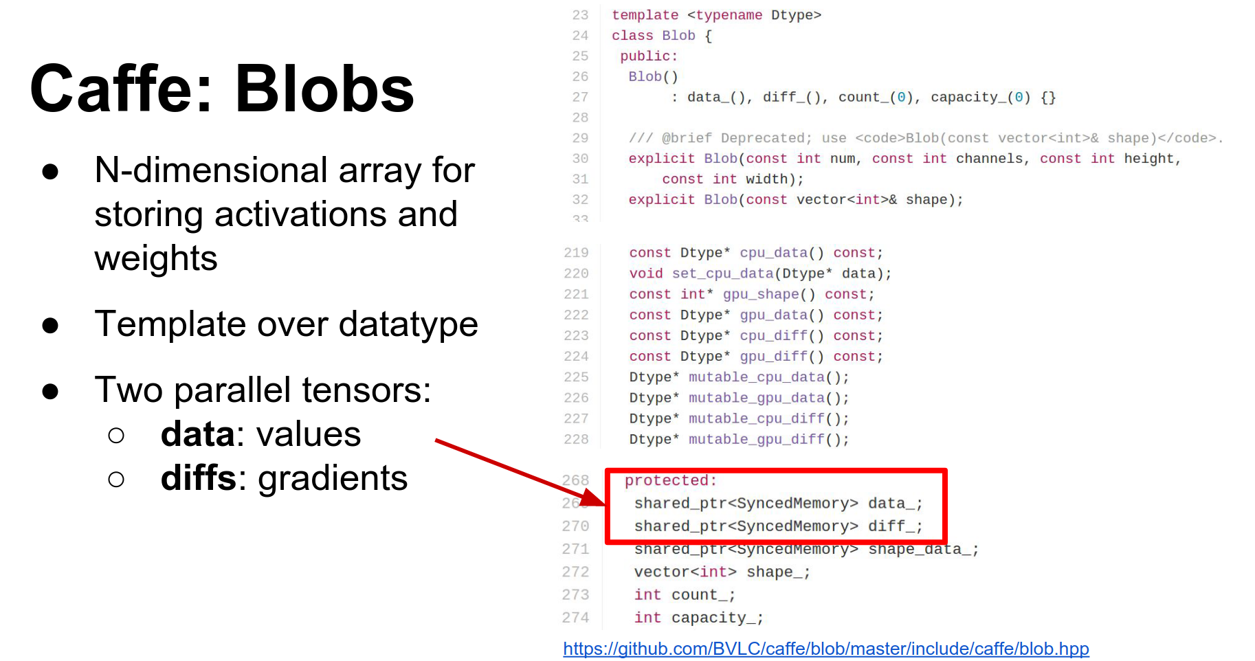
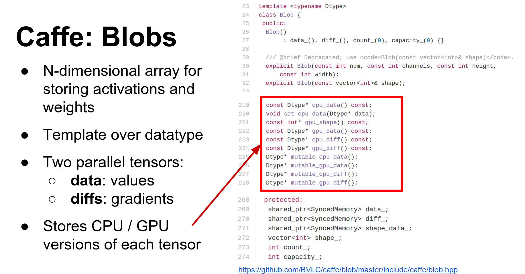
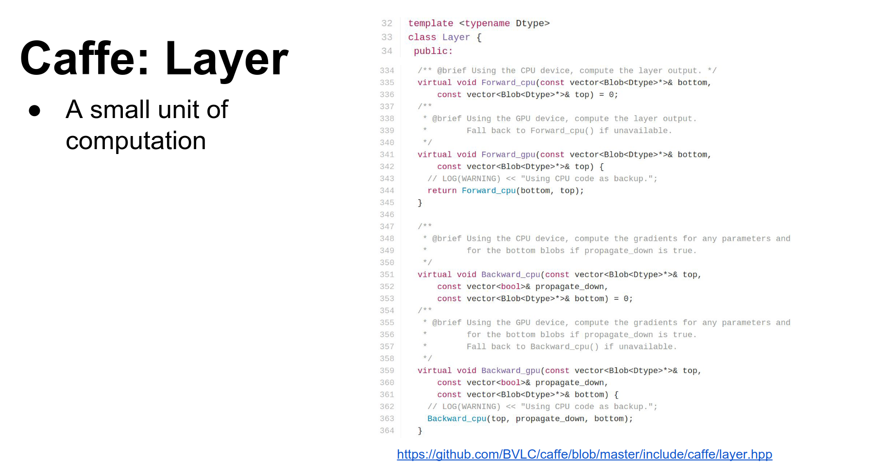
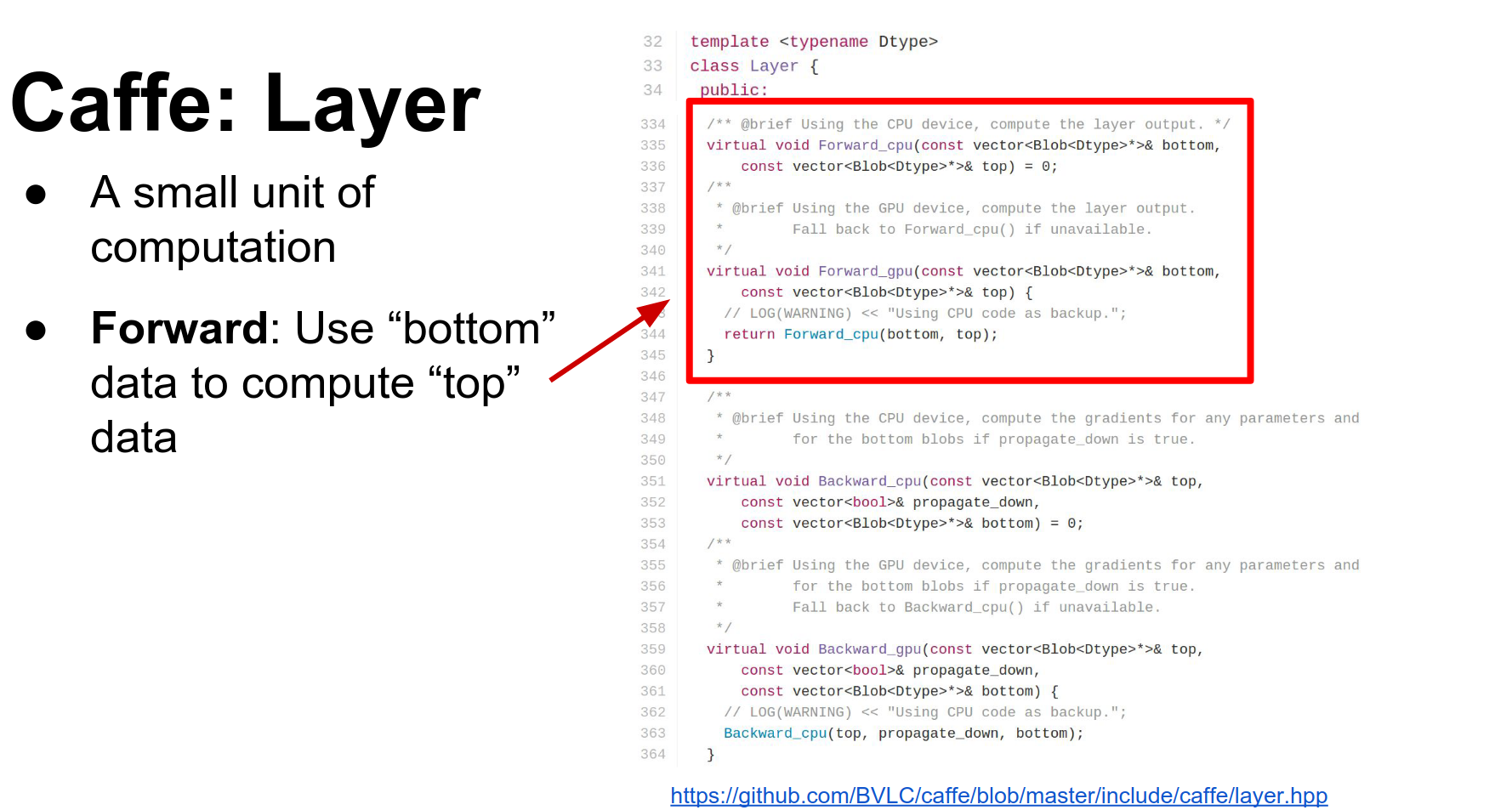
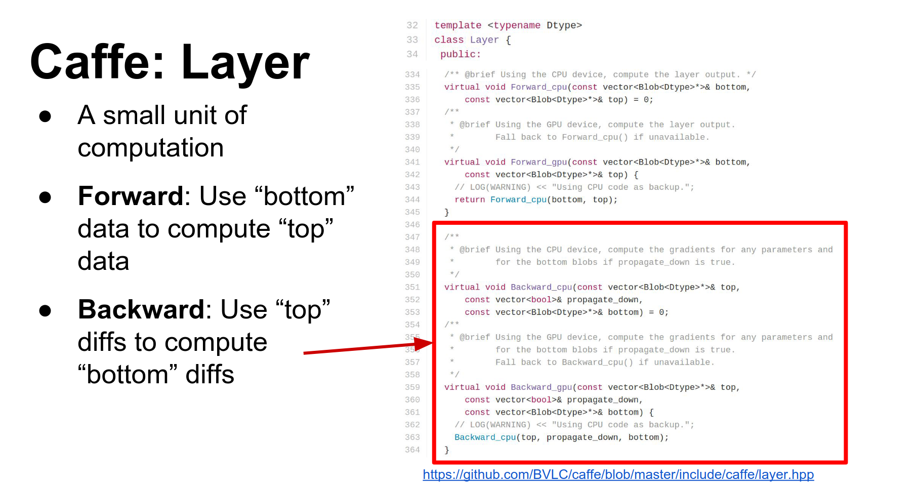
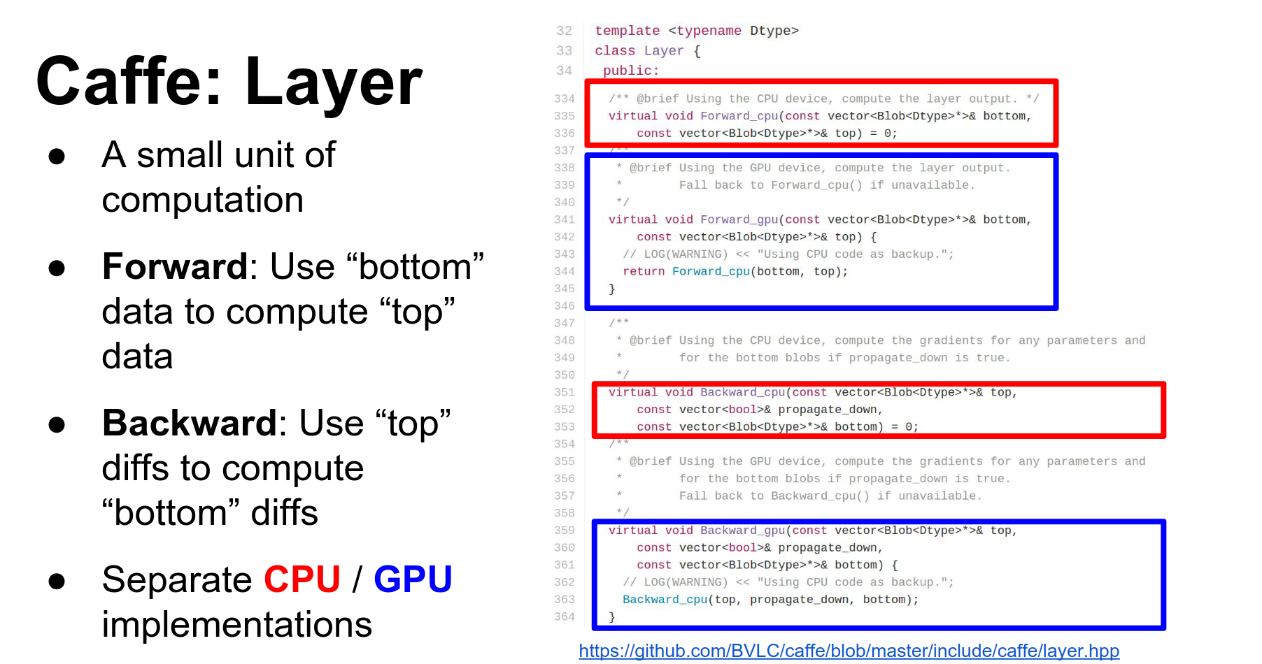
1. Blob: Blobs store all your data, weights, and activations. They are N-dimensional tensors. They actually store two copies: data (raw data) and diff (gradients). They also have CPU and GPU versions of each.
2. Layer: A layer is a function. It receives input blobs (bottoms) and produces output blobs (tops). In the forward pass, it fills the data of the top blobs. In the backward pass, it computes gradients for the bottom blobs.
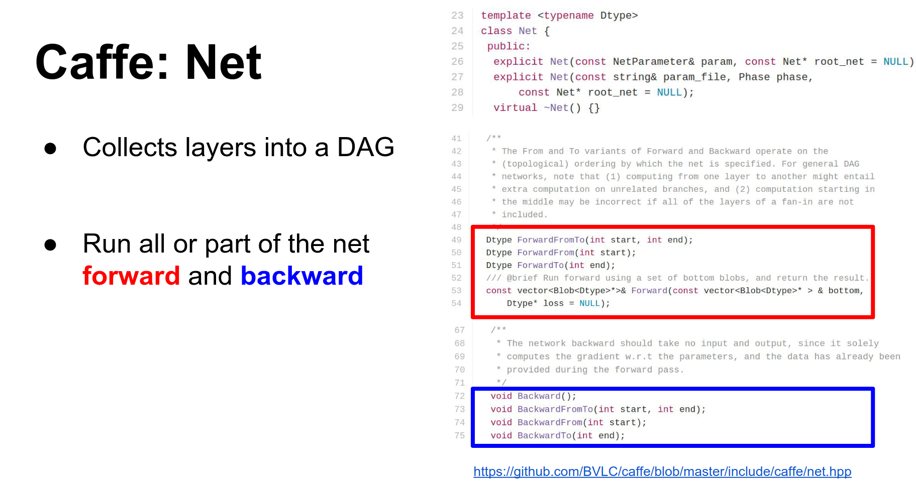
3. Net: A Net combines a bunch of layers. It is a directed acyclic graph of layers and is responsible for running the forward and backward methods in the correct order.
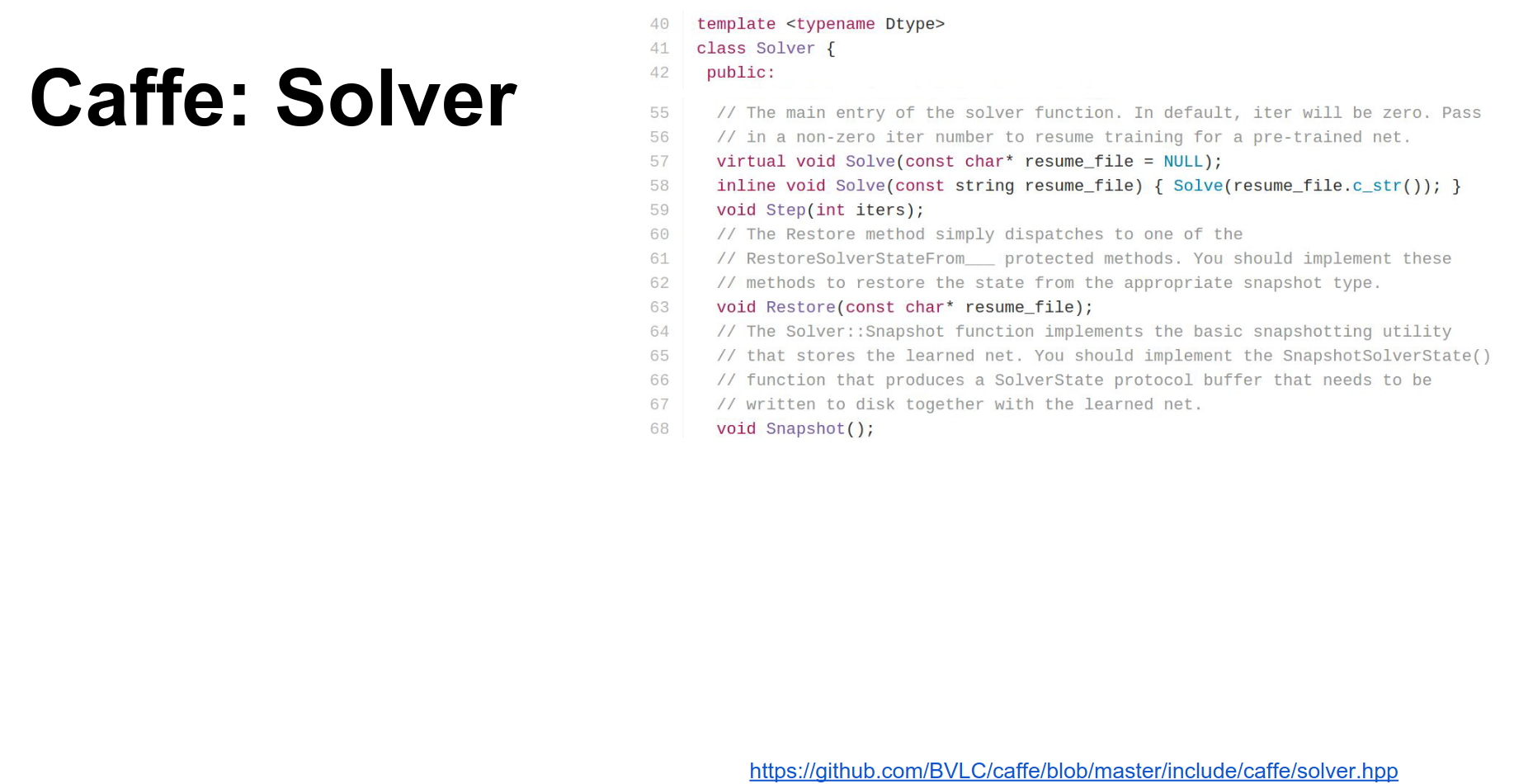
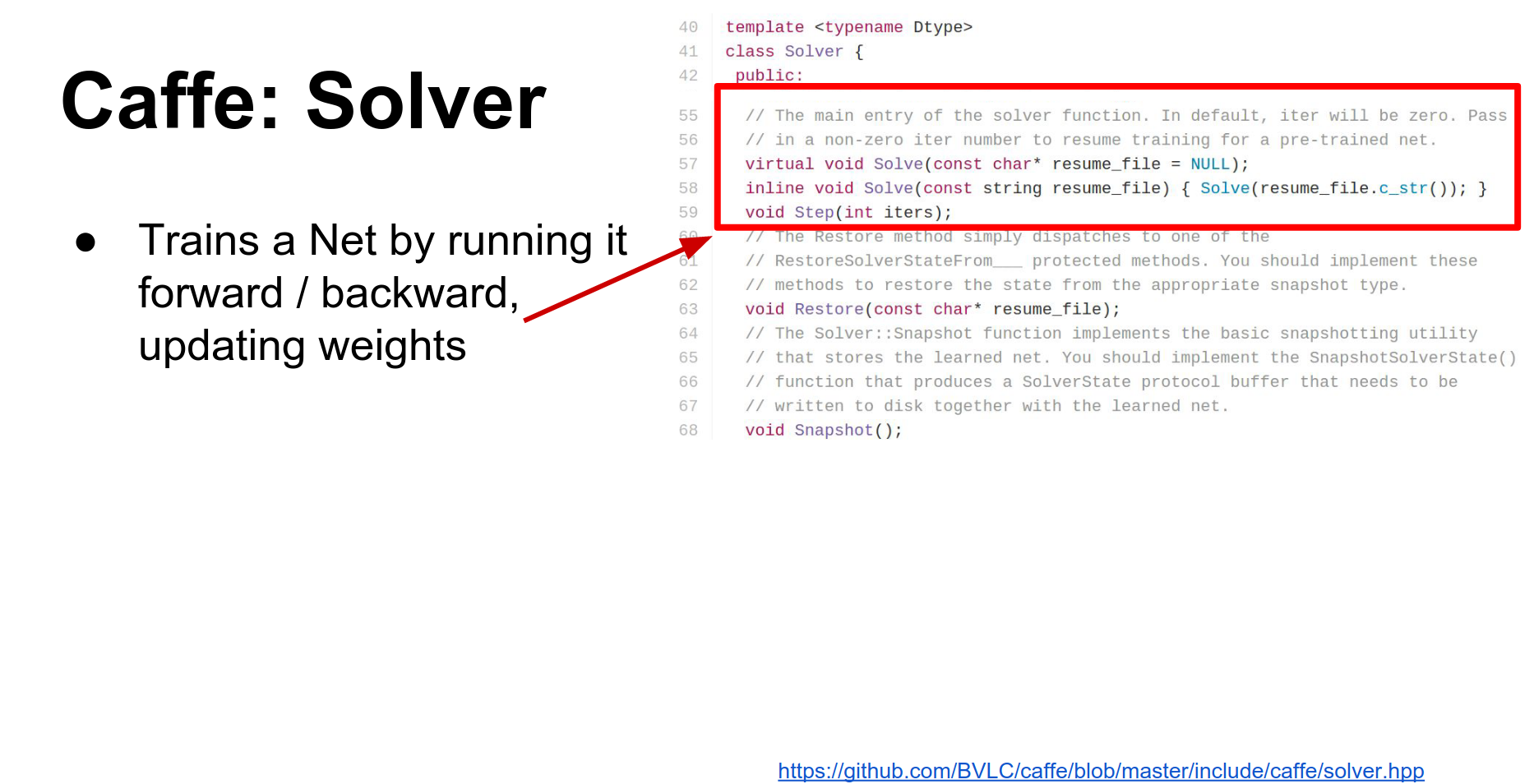
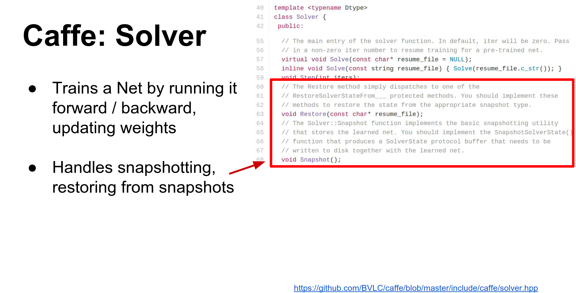
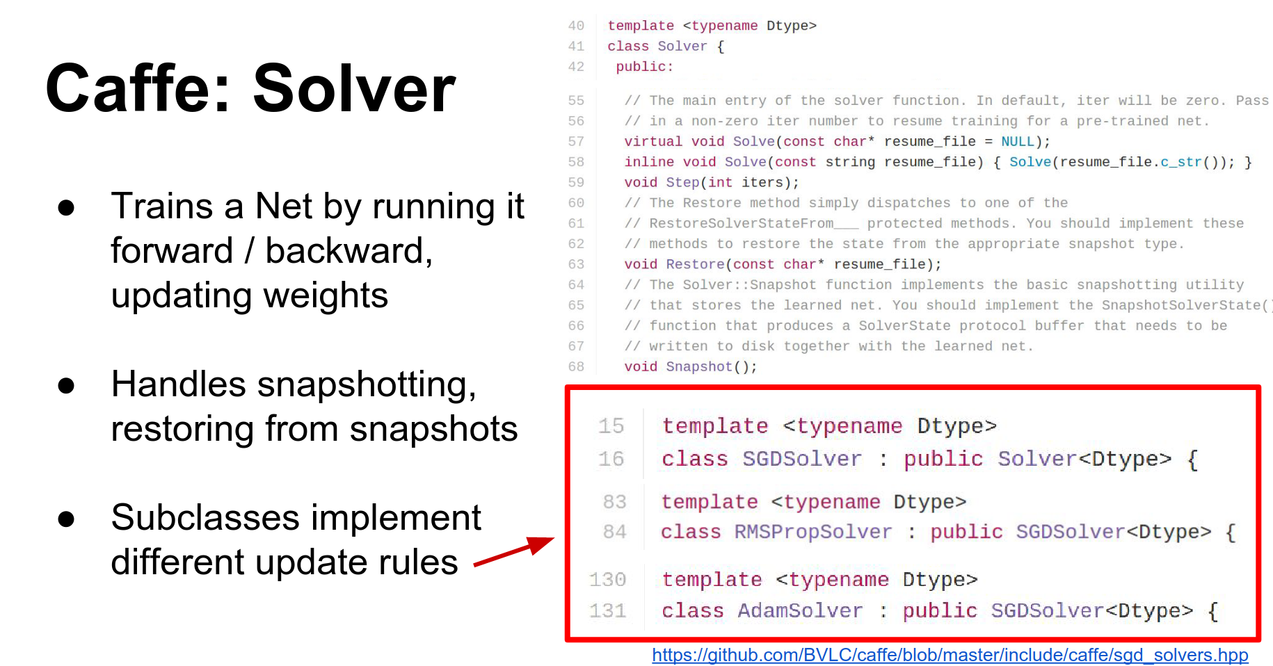
4. Solver: The Solver optimizes the network. It runs the net forward and backward, updates parameters, and handles checkpointing. Different update rules (SGD, Adam, RMSProp) are implemented as subclasses.

This gives you an overview of how things fit together: the Net contains Blobs and Layers, and the whole thing is optimized by a Solver.

Caffe makes heavy use of Protocol Buffers.

Protocol Buffers

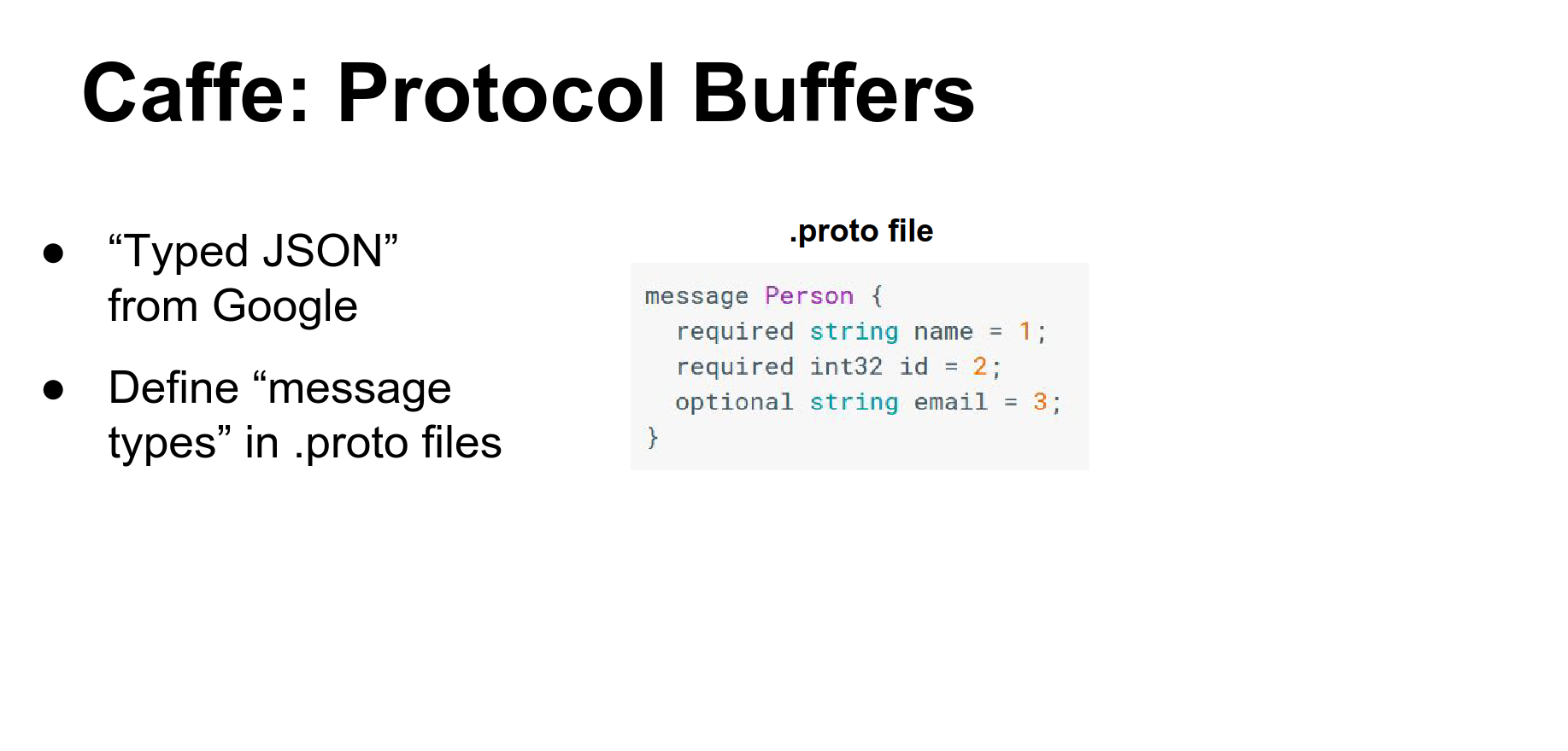
Protocol Buffers are like a binary, strongly-typed JSON used widely inside Google for serializing data.

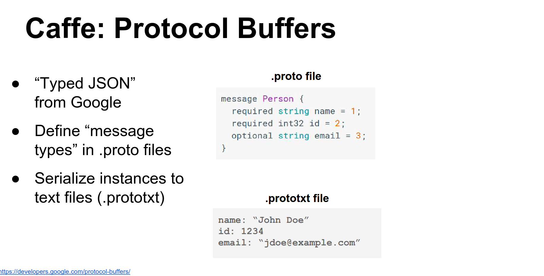
You define a .proto file that specifies the fields of your objects.

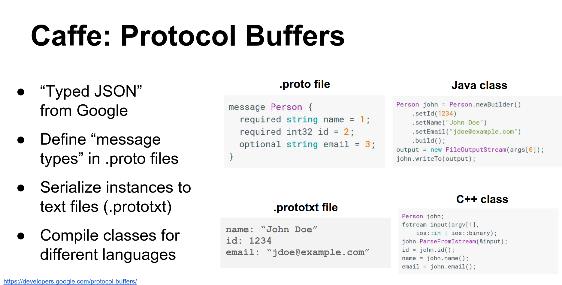
You can serialize instances to human-readable .prototxt files.

The protobuf compiler generates classes in various languages (C++, Python, Java) to access these data types. Caffe uses protocol buffers to store pretty much everything.

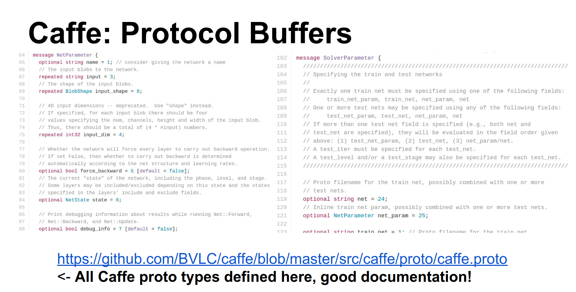
Caffe has one giant file called caffe.proto that defines all the protocol buffer types used in Caffe. It is thousands of lines long but is the most up-to-date documentation. I encourage you to read it.

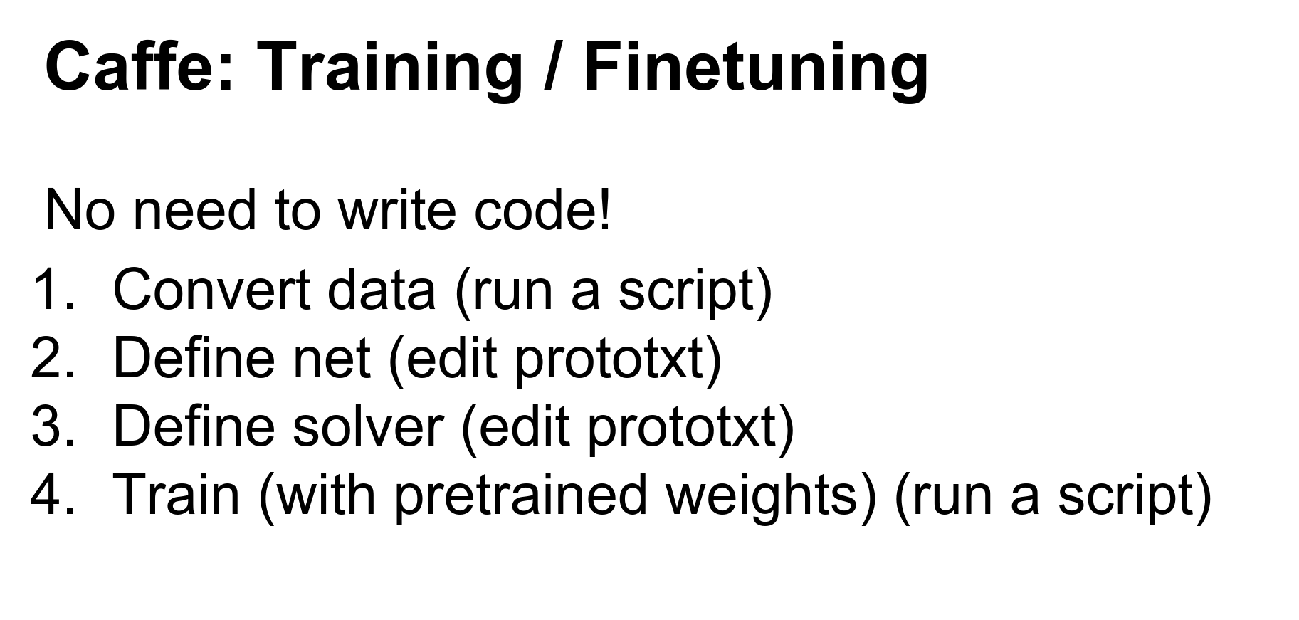
When working with Caffe, you generally have this four-step process:

1. Convert your data: Use existing binaries to convert images to Caffe's format.
2. Define your Net: Write a .prototxt file defining the architecture.
3. Define your Solver: Write a .prototxt file defining the optimization parameters.
4. Train: Pass these files to the caffe train binary.

This will spit out your trained Caffe model to disk.

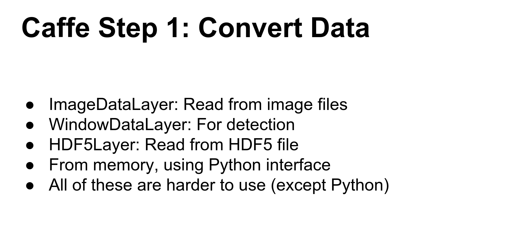
Step 1: Convert Data. Caffe uses LMDB by default. If you have images and labels, Caffe has a script to convert them into a giant LMDB file.

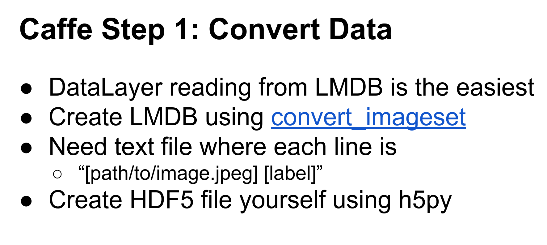
Caffe has other options (HDF5, reading directly from memory), but LMDB is the easiest to work with in the Caffe ecosystem.

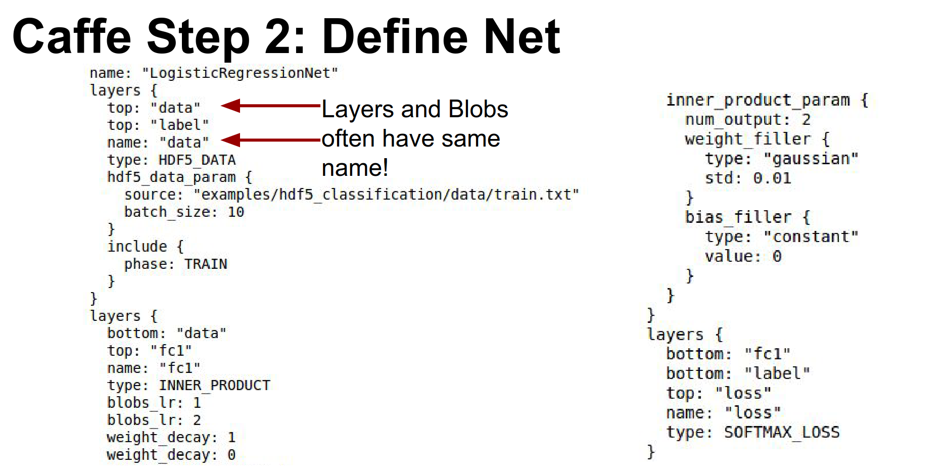
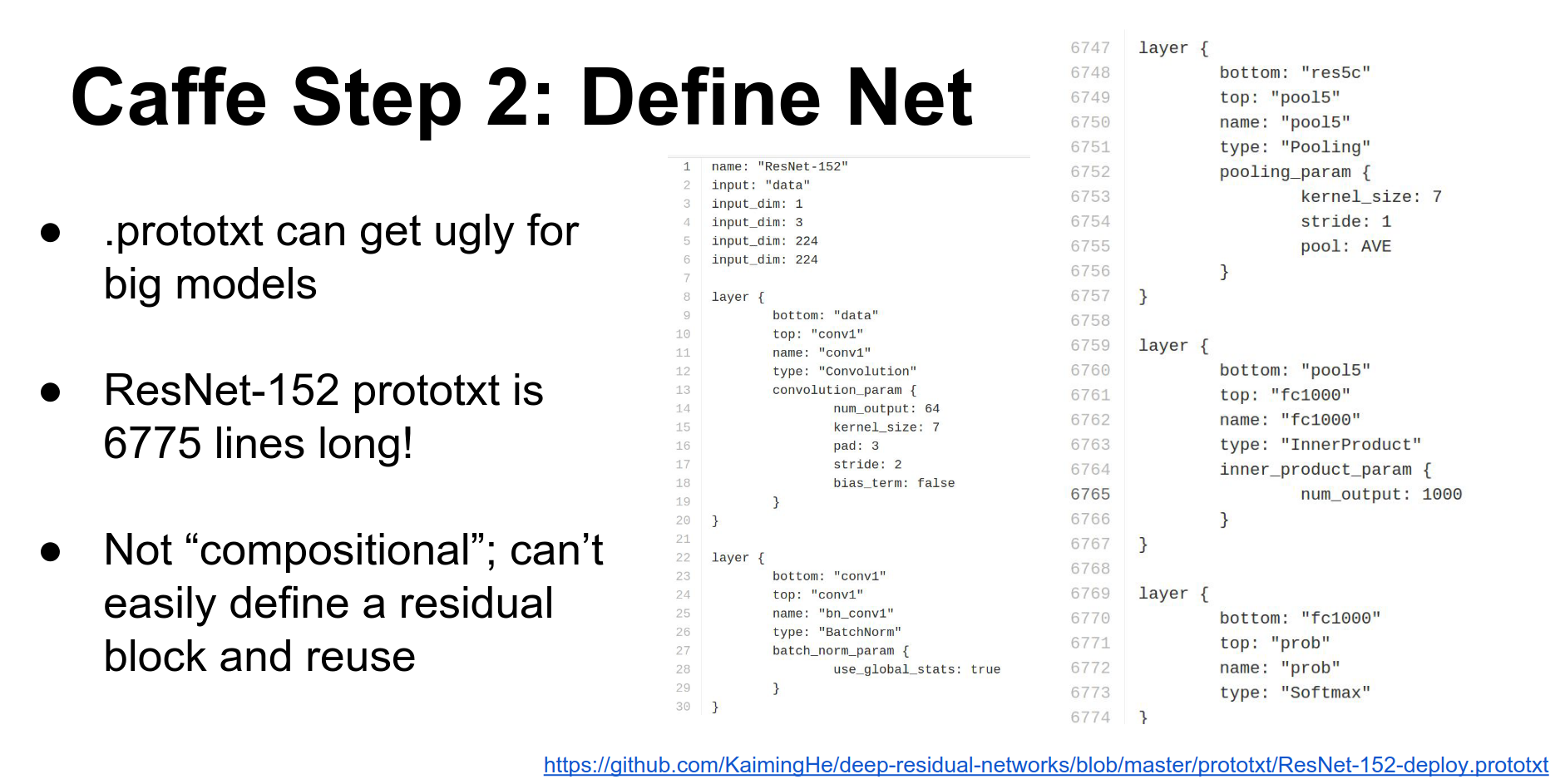
Step 2: Define Net. You write a big .prototxt.

Here is a simple model for logistic regression. It reads data, has a fully connected layer (called InnerProduct in Caffe), and a Softmax loss.

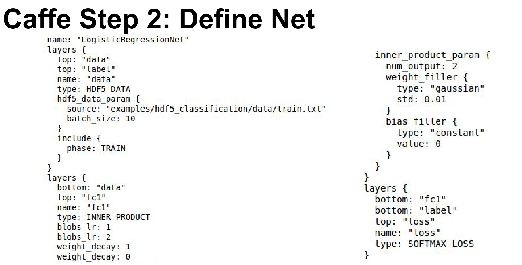
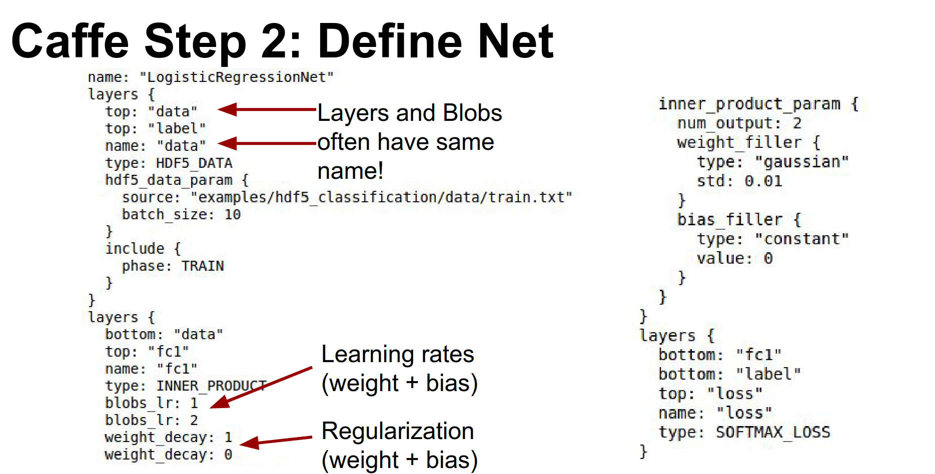
Every layer typically includes blobs to store data, gradients, and weights. The layer's blobs and the layer itself typically have the same name.

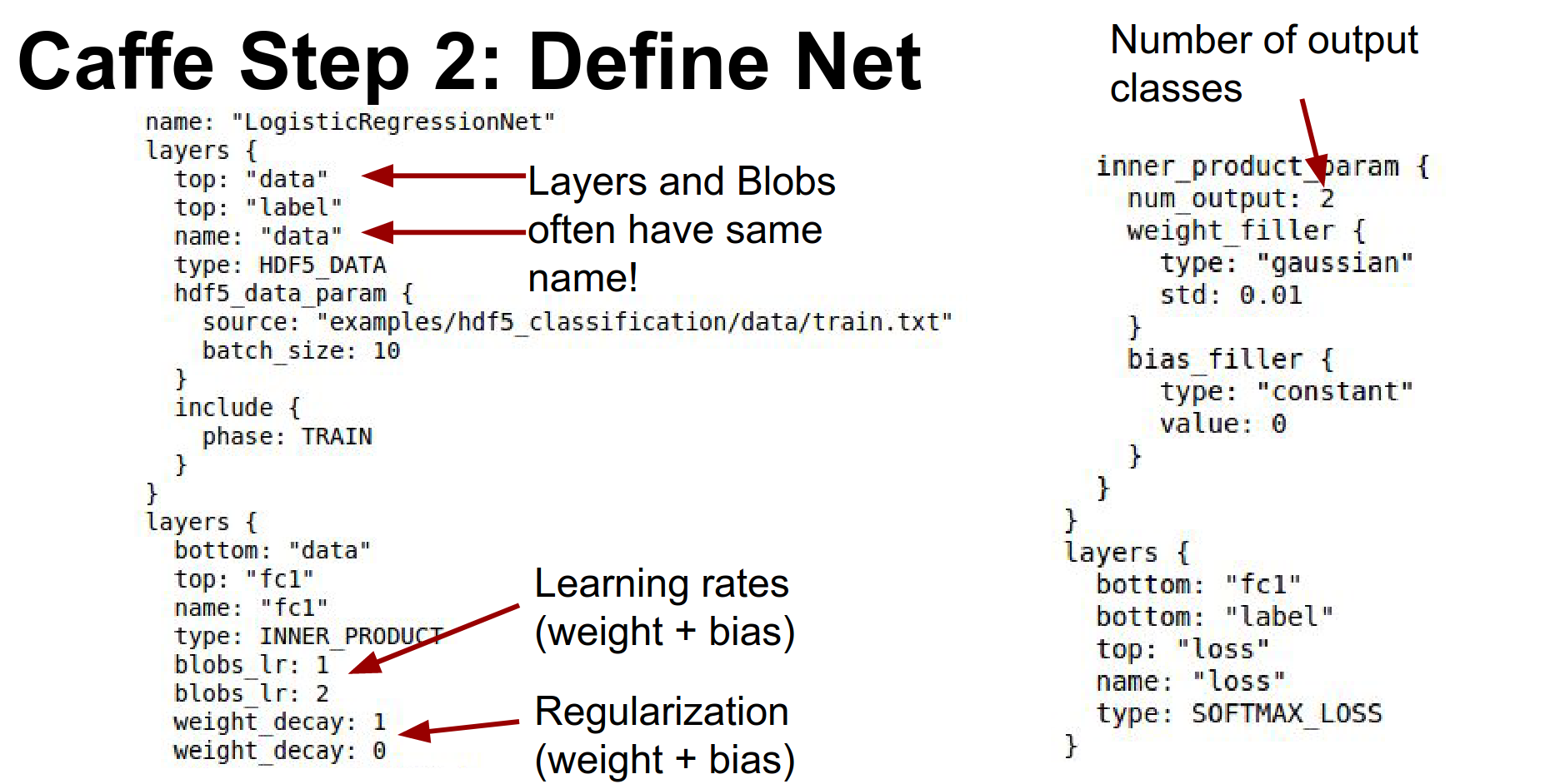
You define learning rates for weights and biases directly in the layer definition (lr_mult).

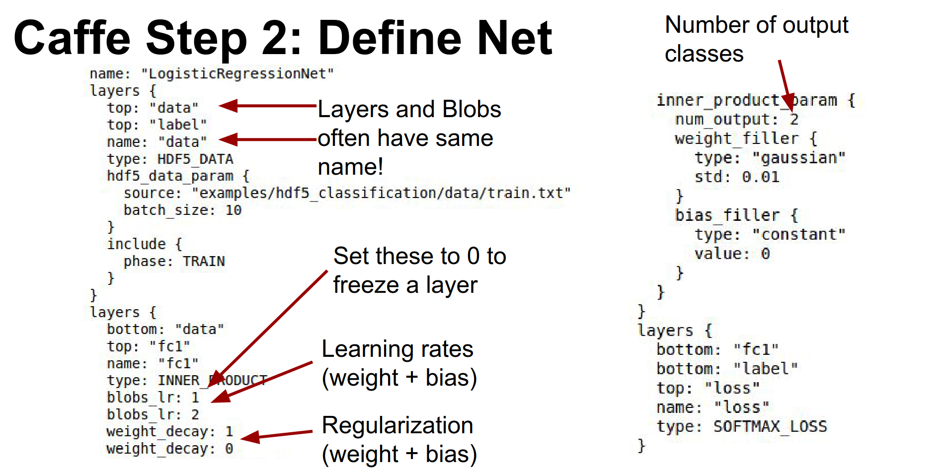
The number of output classes is specified in num_output.

To freeze layers, you set the learning rate multipliers to zero.

For large models like ResNet or GoogLeNet, the .prototxt can get out of hand (ResNet's is almost 7,000 lines). Caffe doesn't support compositionality well, so people often write Python scripts to generate these files.

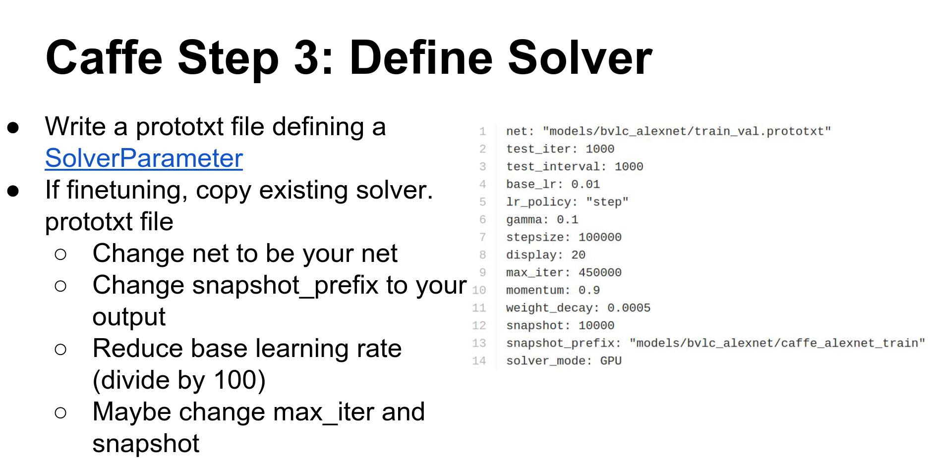
Fine-tuning: You typically download an existing .prototxt and a .caffemodel weights file.

The .caffemodel file is a binary containing key-value pairs matching layer names to weights.

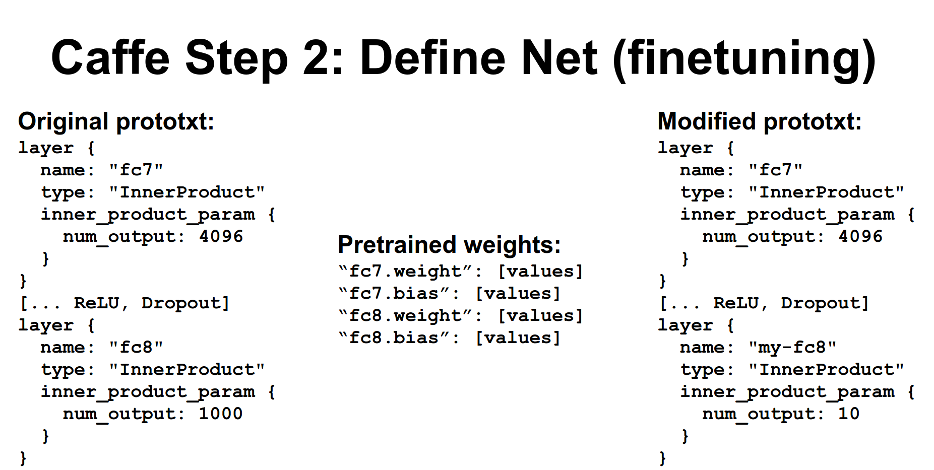
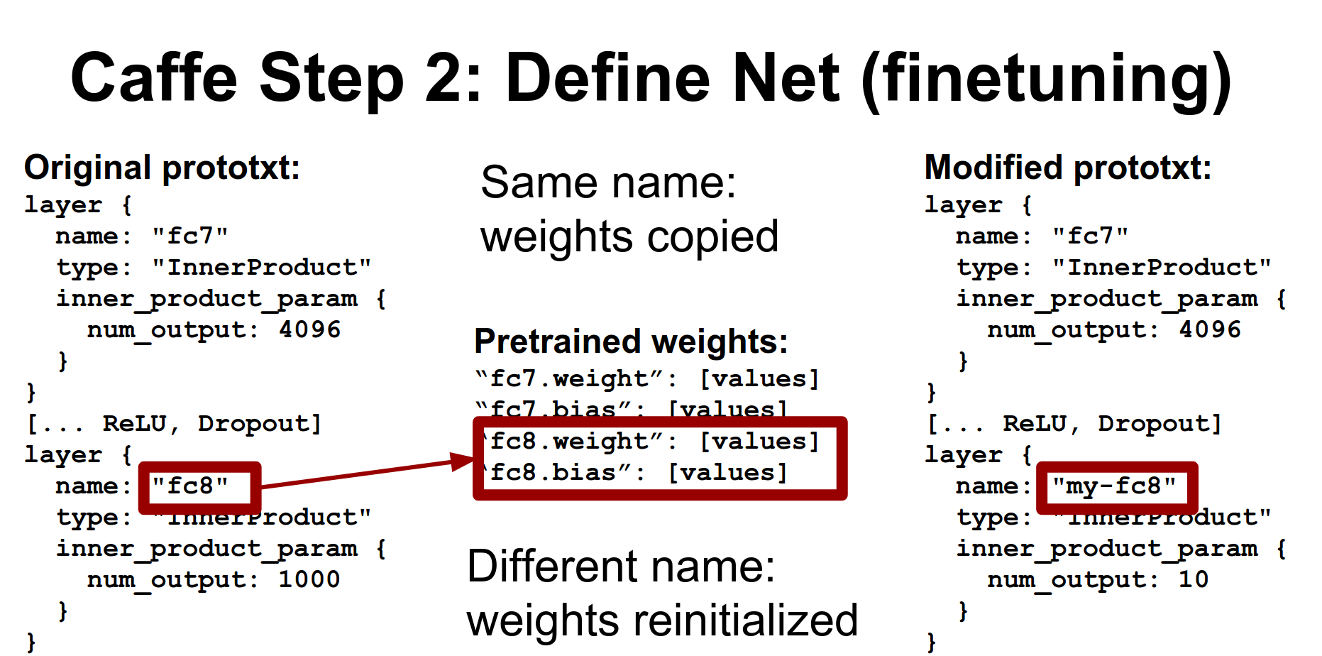
When you load a model, Caffe tries to match names. If names match, weights are initialized from the file.

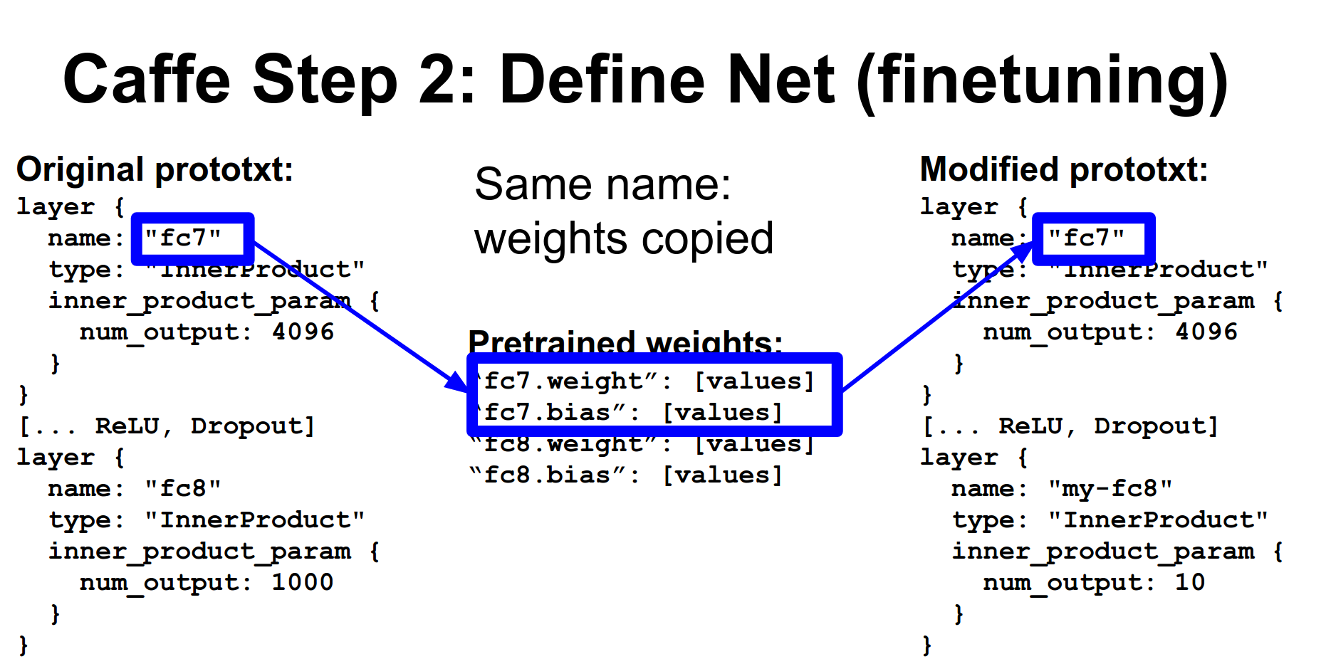
If names don't match, layers are initialized from scratch. This is how you reinitialize the output layer for a new task (e.g., changing from 1000 ImageNet classes to 10 classes): just change the layer name in the .prototxt.

Step 3: Define Solver. This is another .prototxt defining learning rate, decay, checkpointing, etc.

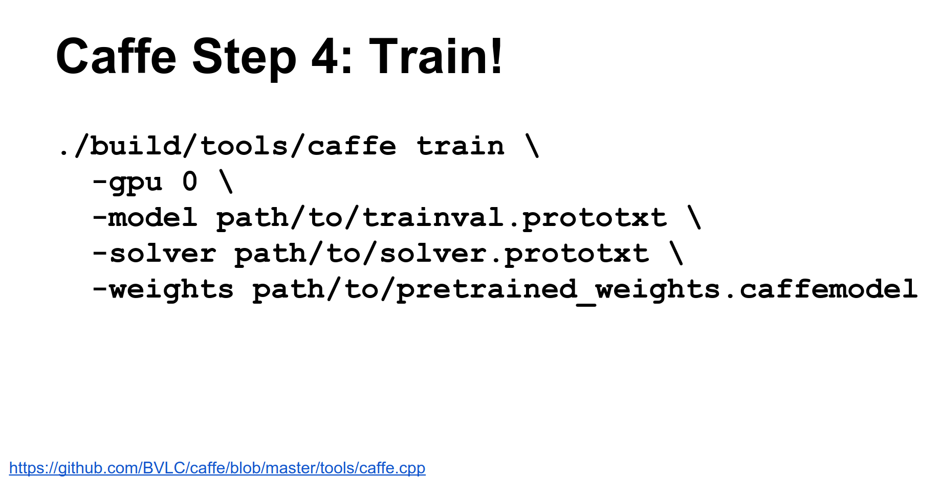
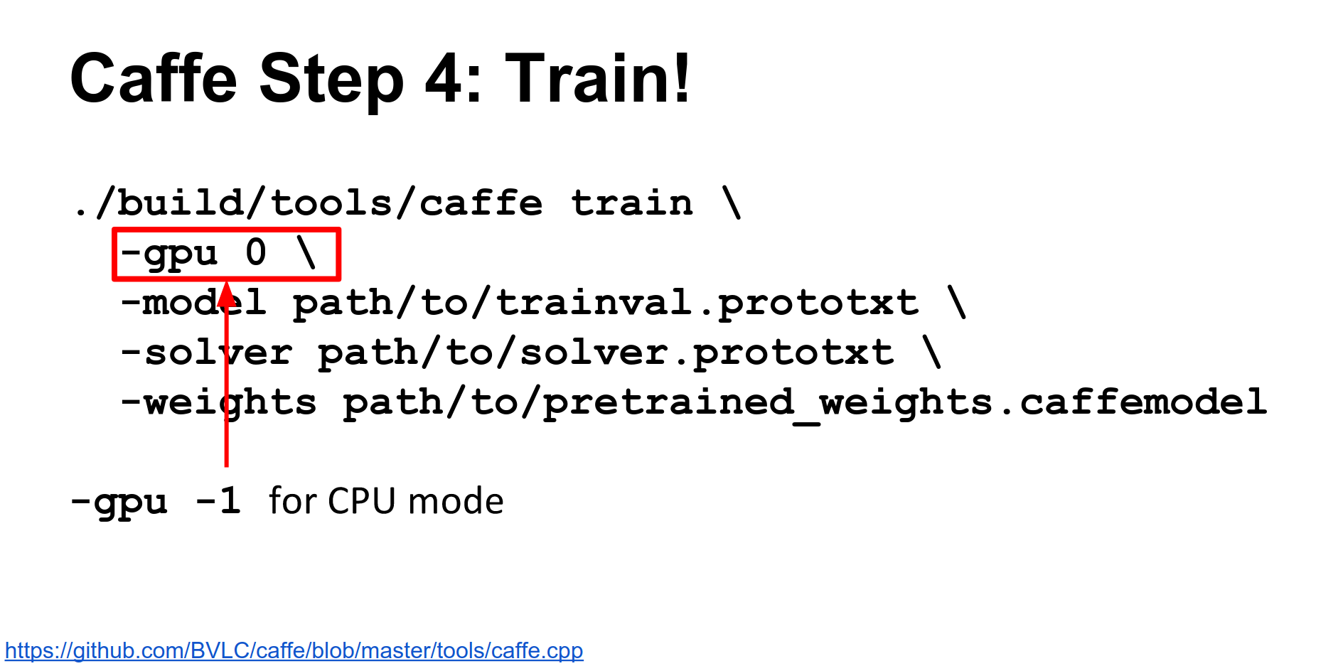
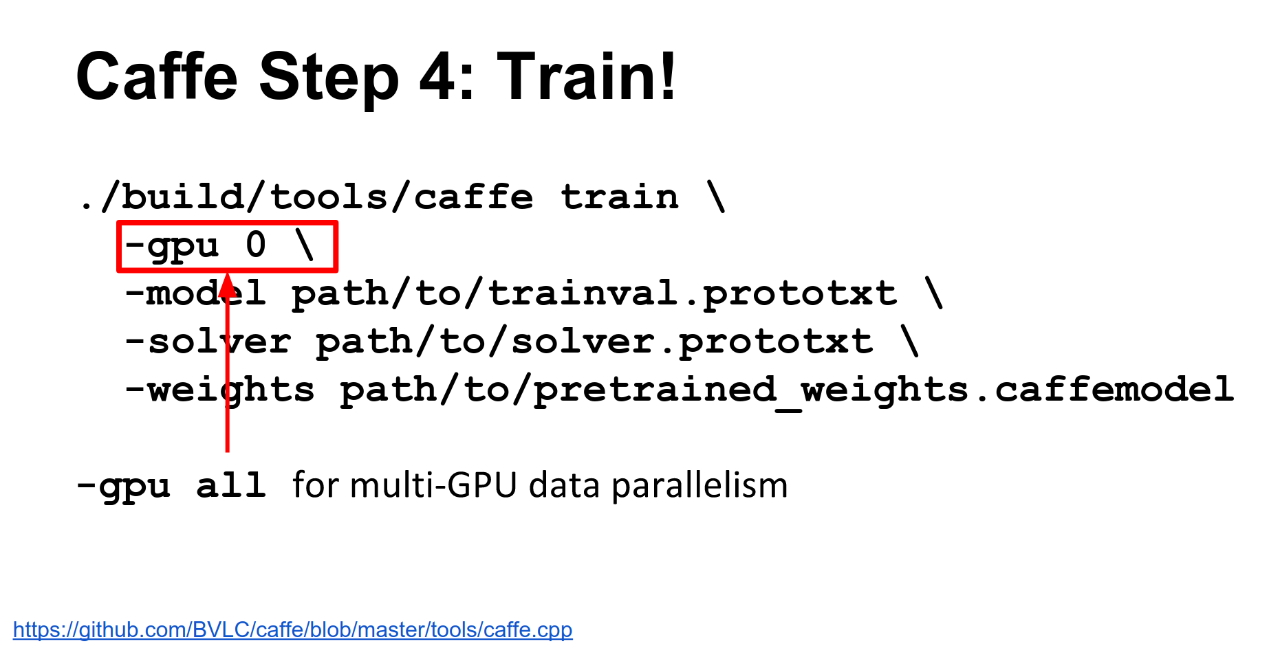
Step 4: Train. Call the caffe train binary with your solver and weights.

You can specify which GPU to run on, or use -1 for CPU only.

Caffe supports data parallelism. You can pass multiple GPU IDs or -gpu all to automatically split mini-batches across GPUs.

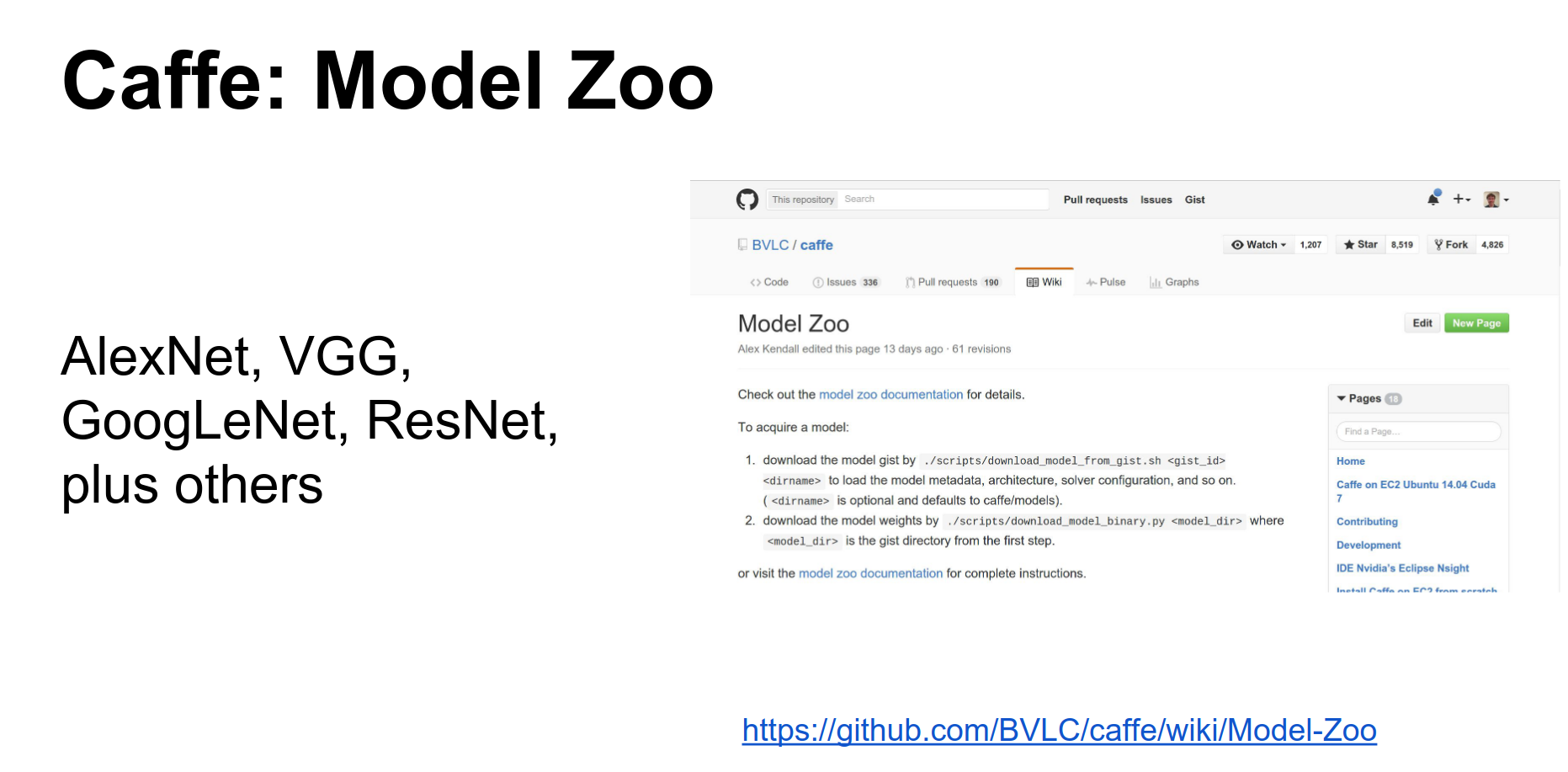
Model Zoo: Caffe has a great Model Zoo where you can download pre-trained models (AlexNet, VGG, ResNet, etc.). This is a really strong point of Caffe.

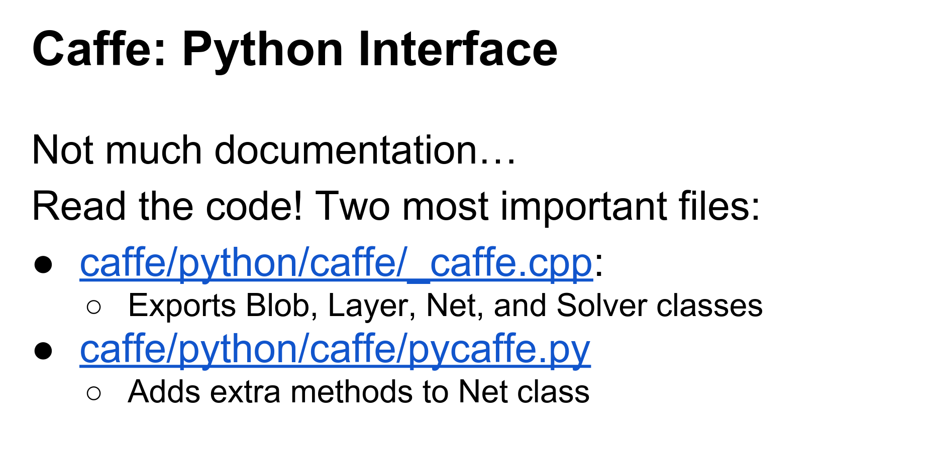
Python Interface: Caffe has a Python interface (PyCaffe). It's useful but documentation is sparse; read the code.

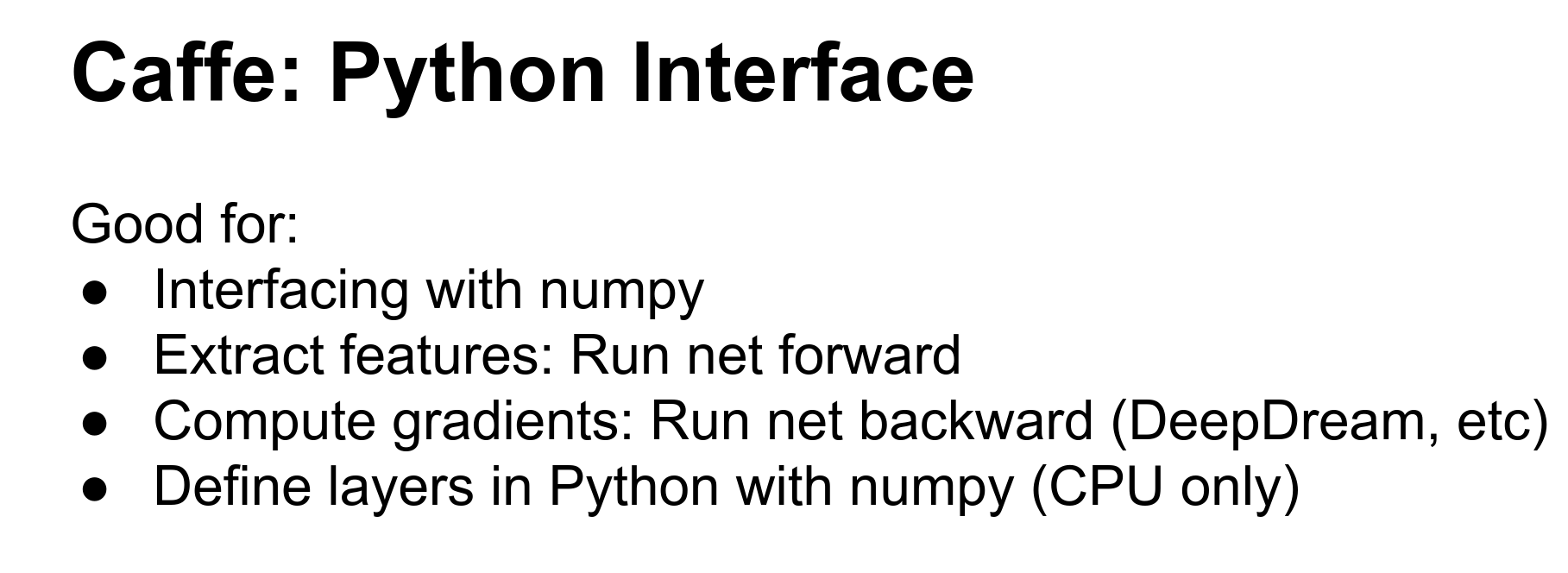
The Python interface lets you do complex initialization, run networks forward/backward with numpy arrays (great for DeepDream or visualization), and extract features.

You can also define layers in Python, but they will be CPU-only, which incurs communication overhead.

Caffe Pros and Cons:

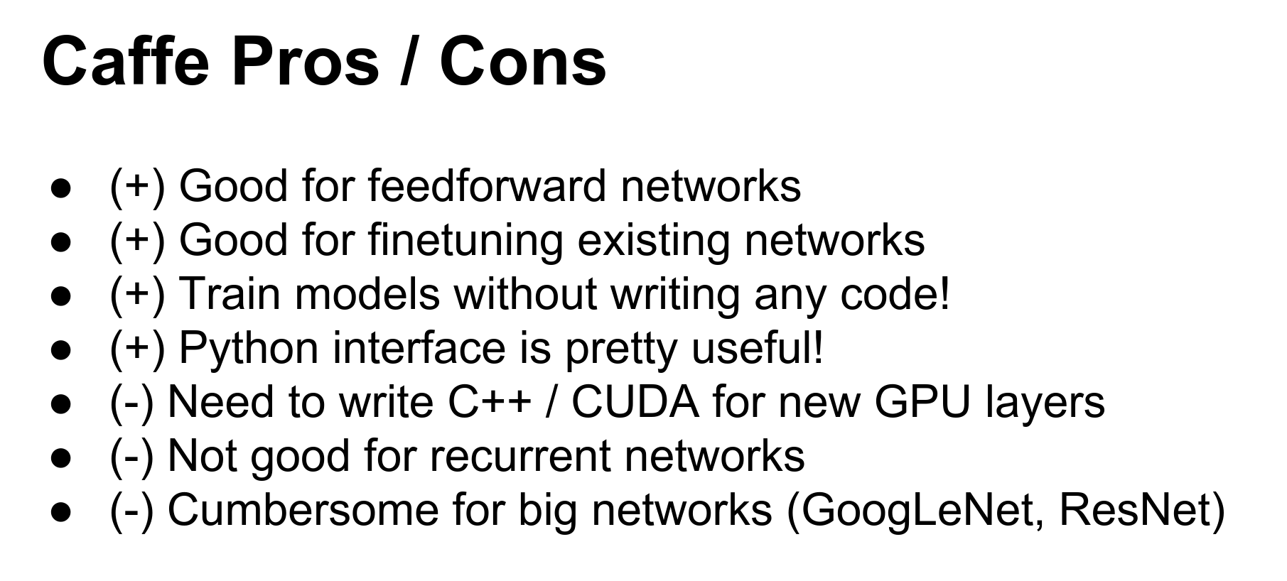
• Pros: Good for feed-forward networks, no code required, great Model Zoo, Python interface for feature extraction.
• Cons: Cumbersome for big networks (ResNet) or RNNs, writing new layers requires C++ and CUDA.

Can you do cross-validation? In the train/val .prototxt, you can define training and testing phases.

Torch

Torch is my personal favorite. It is from NYU, written in C and Lua, and used a lot at Facebook and DeepMind.

The big thing that freaks people out is Lua.

Lua is a high-level scripting language, similar to JavaScript. It uses Just-In-Time (JIT) compilation, so loops are actually fast (unlike Python). It uses prototypical inheritance (like JavaScript).

It is 1-indexed, which is annoying, but otherwise easy to pick up.

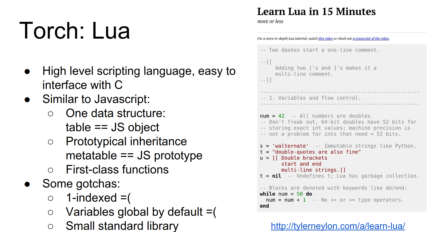
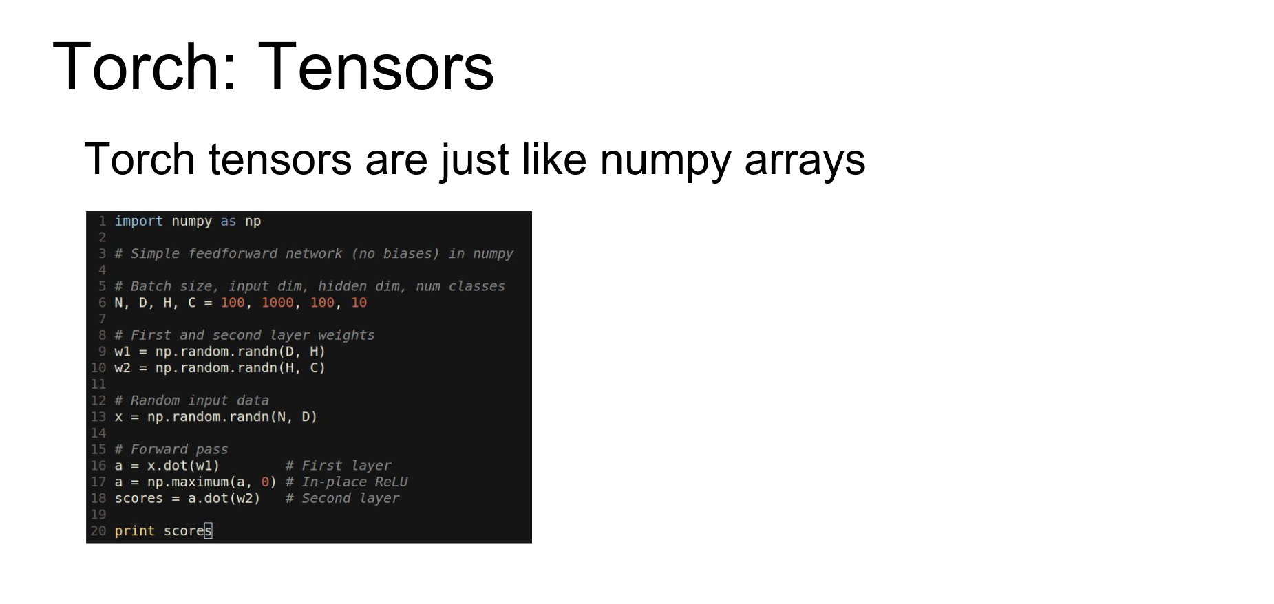
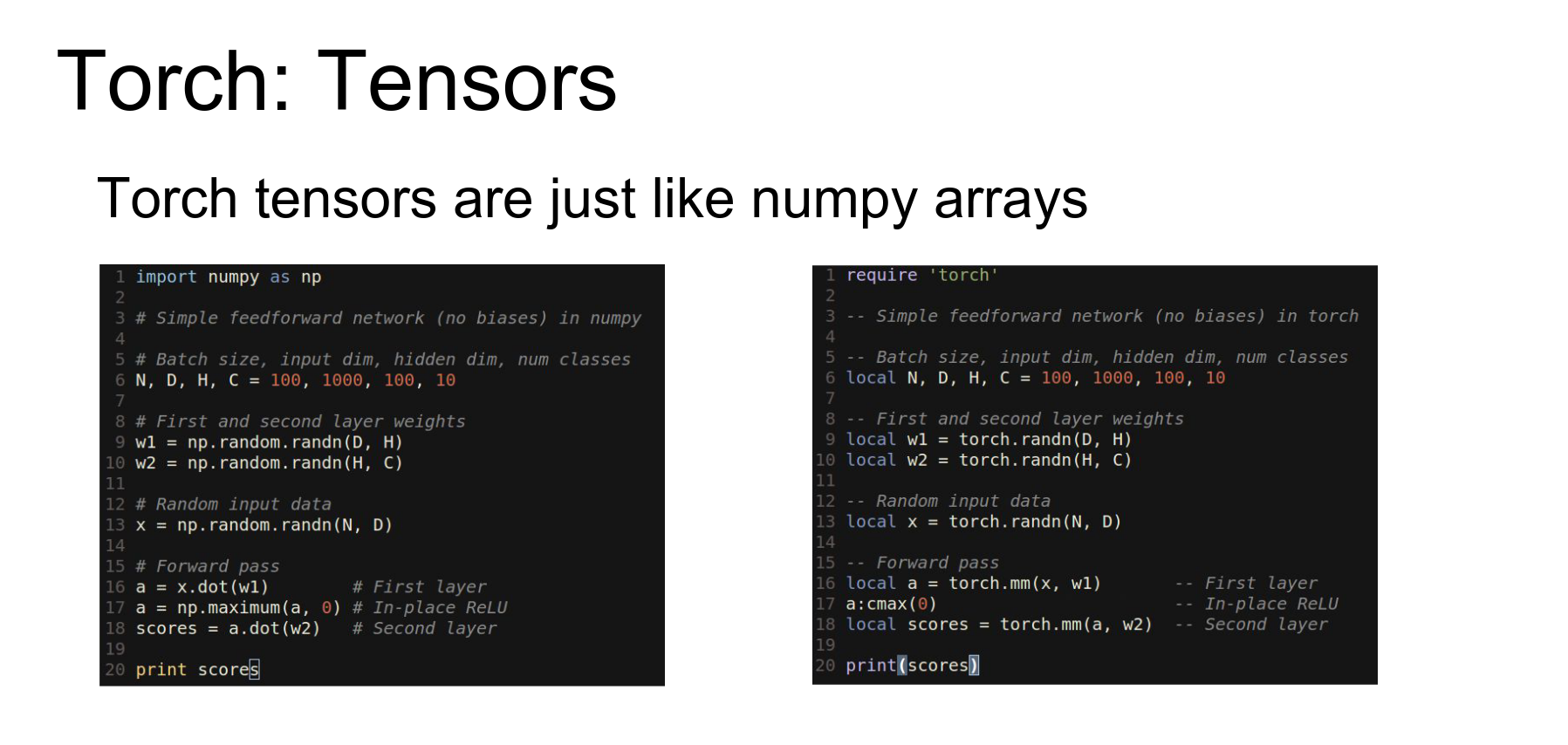
The main idea behind Torch is the Tensor class. It is very similar to a numpy array.

Here is numpy code for a two-layer ReLU network.

Here is the exact same code using Torch tensors in Lua. It's almost a line-by-line translation.

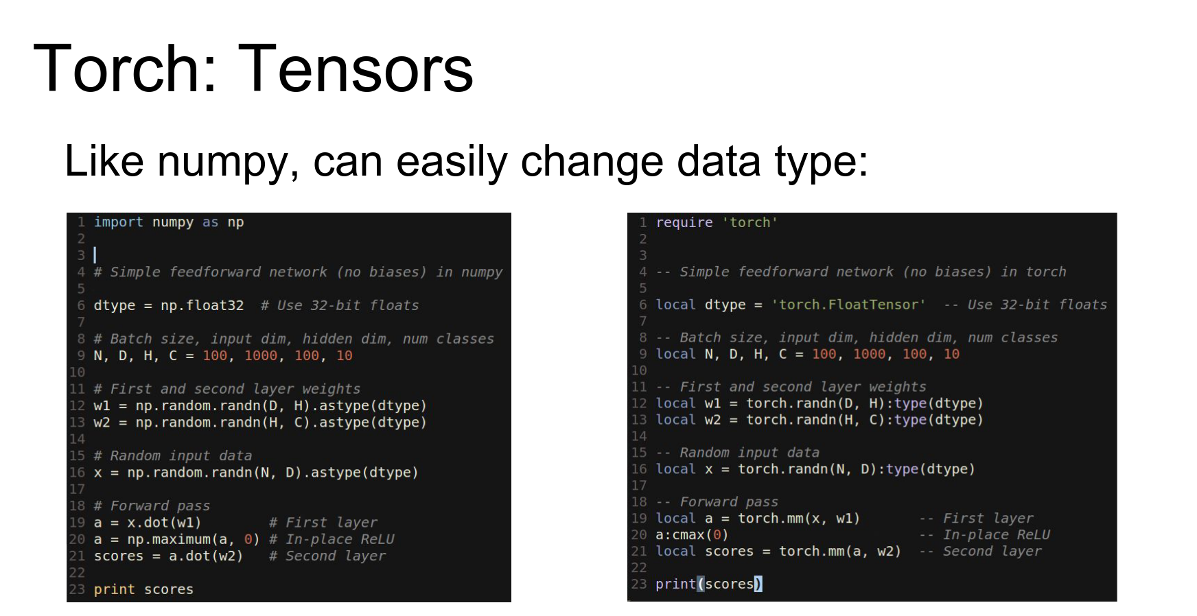
In Torch, changing data types is easy (just like casting in numpy).

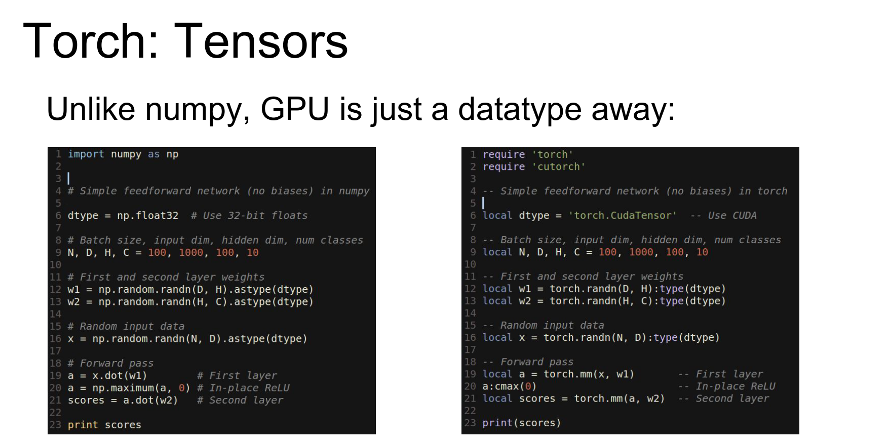
The real reason Torch is great is that the GPU is just another data type.

To run on GPU, you import cutorch and cast your tensors to torch.CudaTensor. Now they live on the GPU.

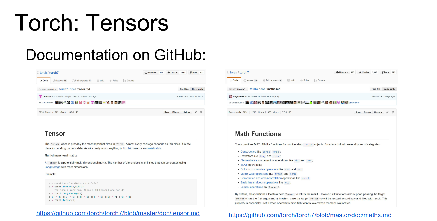
Tensors are like numpy arrays. Documentation is decent.

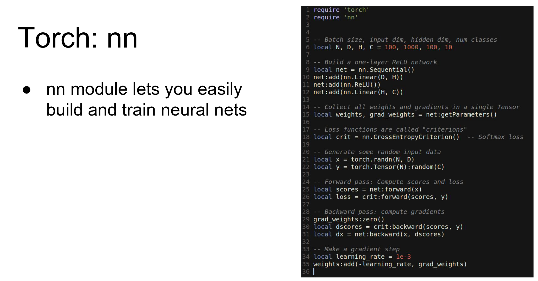
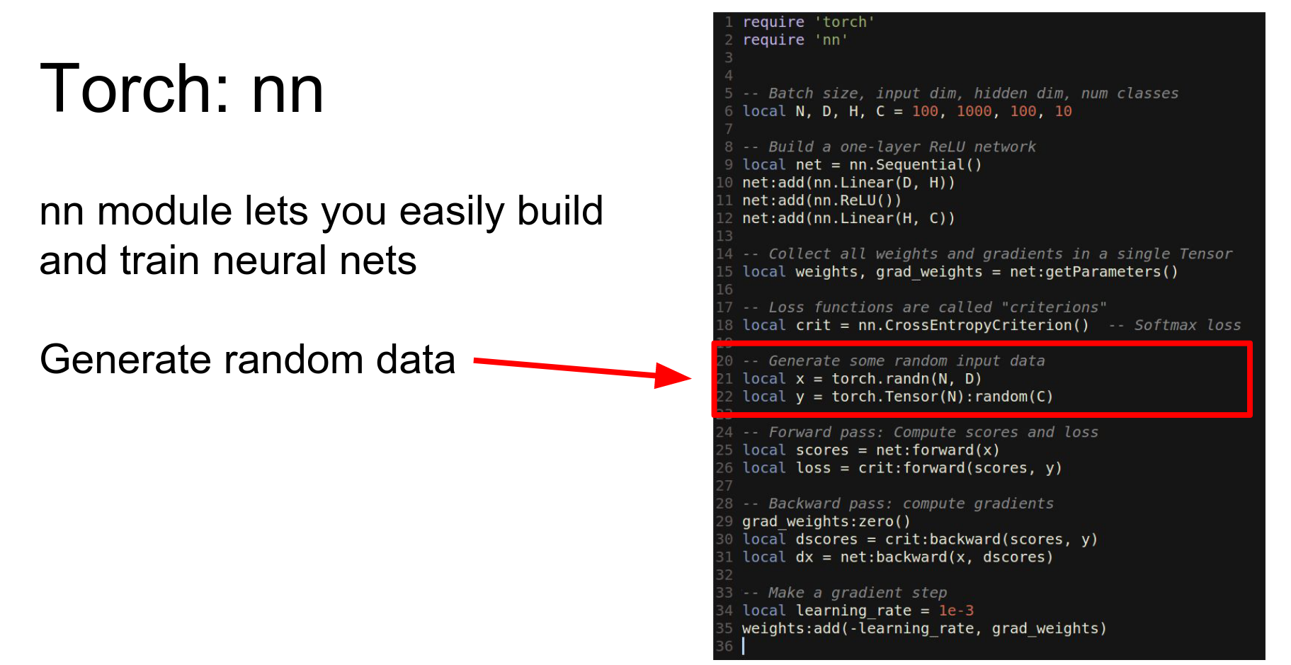
In practice, you use the nn (Neural Network) package. This is a wrapper defining a neural network package in terms of tensors.

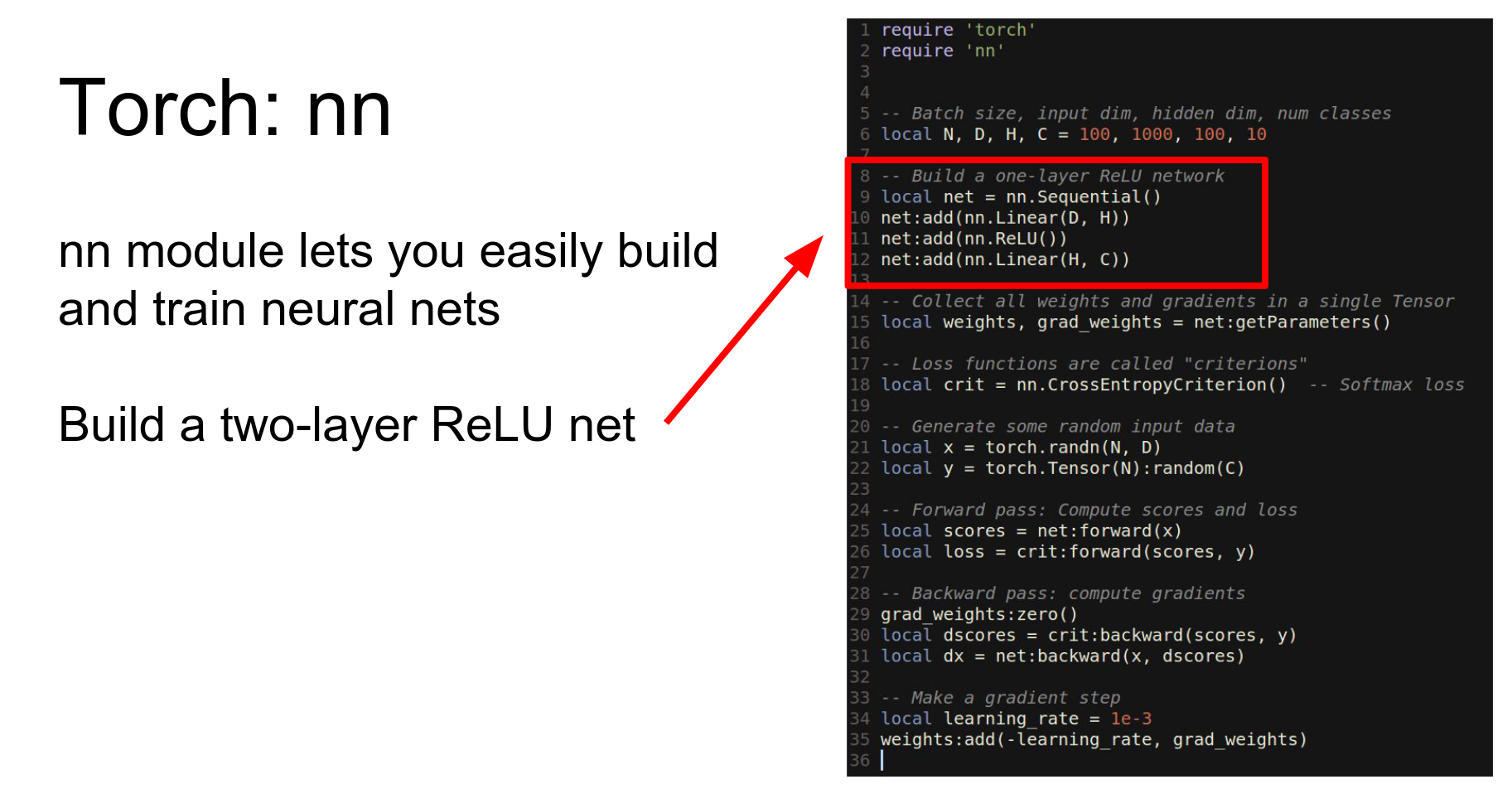
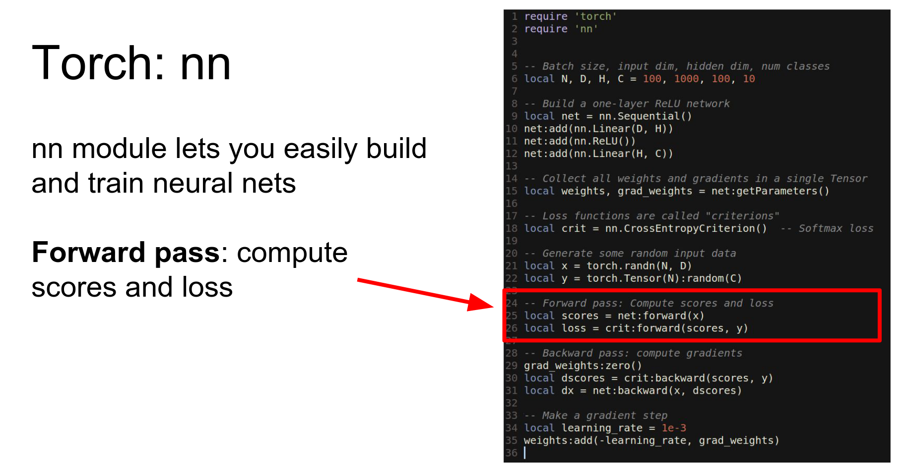
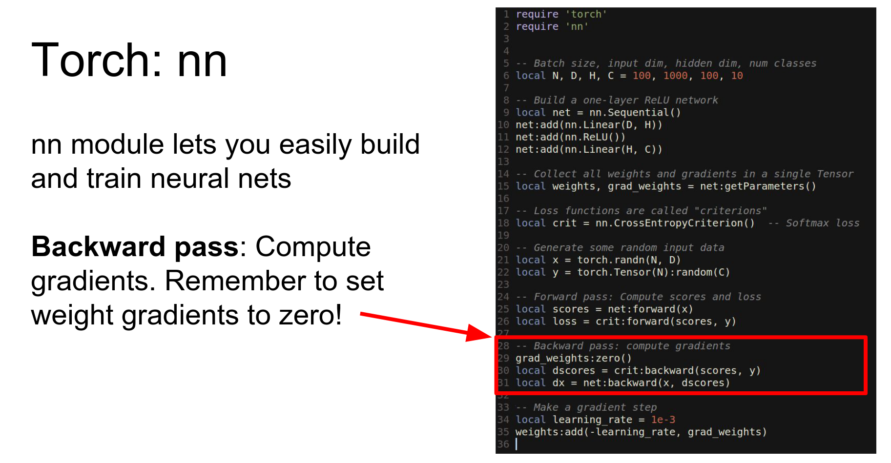
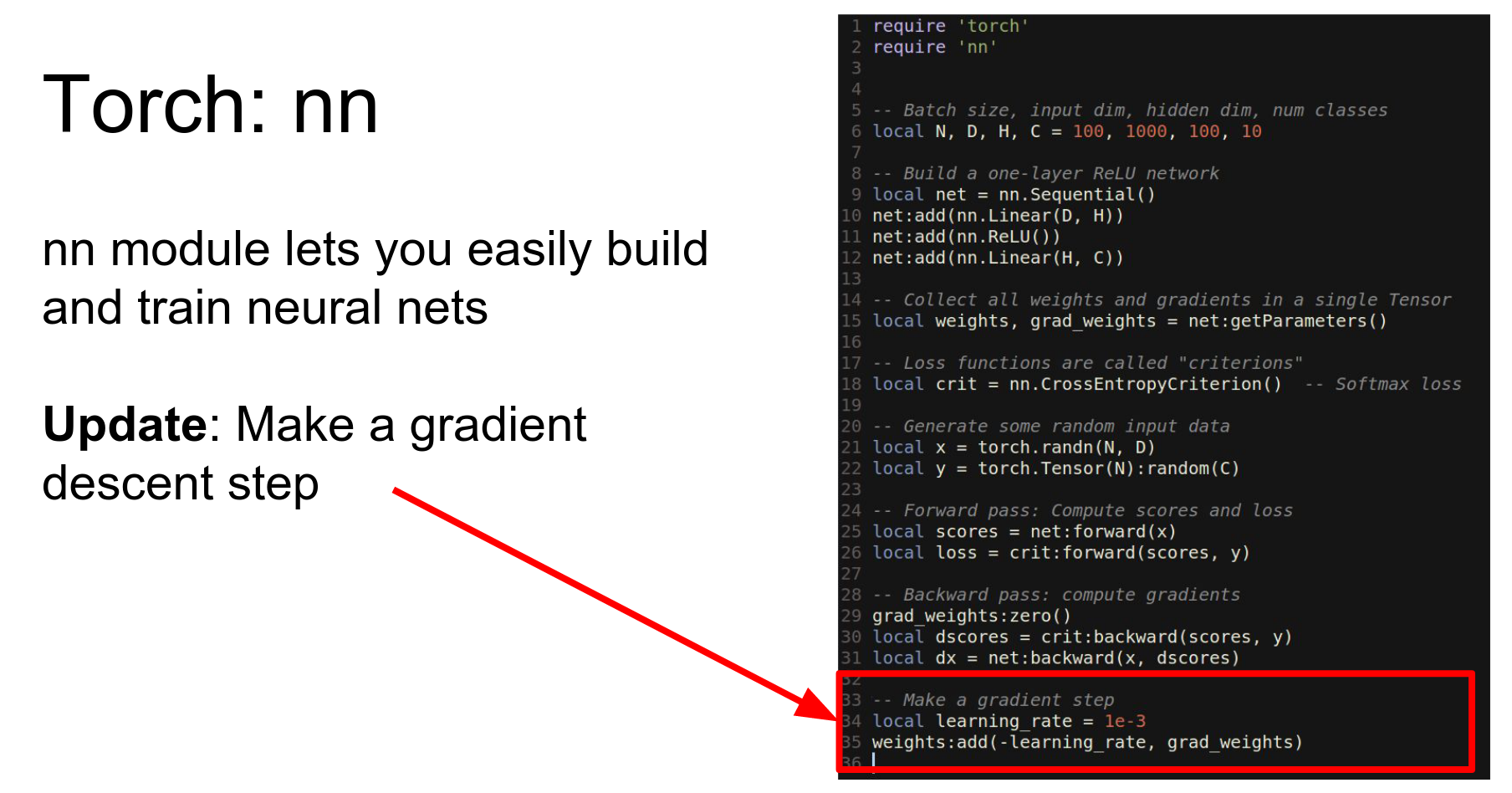
Here is the same two-layer network using nn.

• Define network as Sequential.
• Add Linear and ReLU layers.
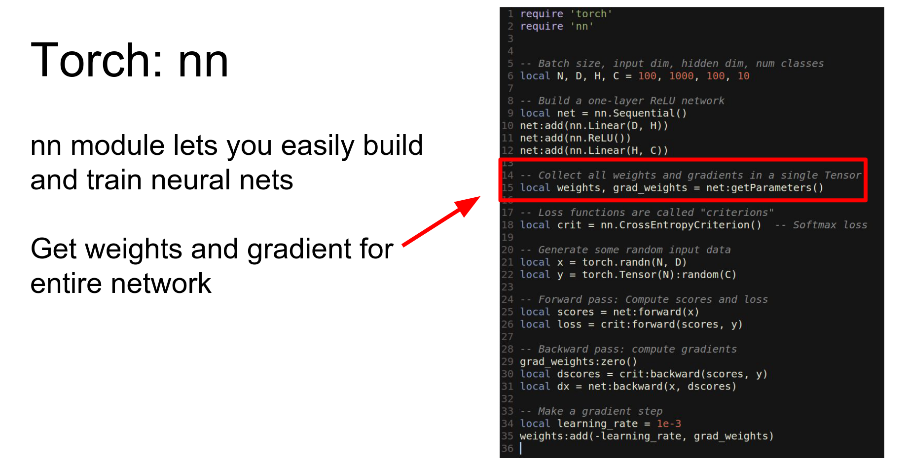
• Use getParameters to get weights and gradients.
• Call forward and backward.
• Update weights.

We have a net.

We have weights grad_weights.

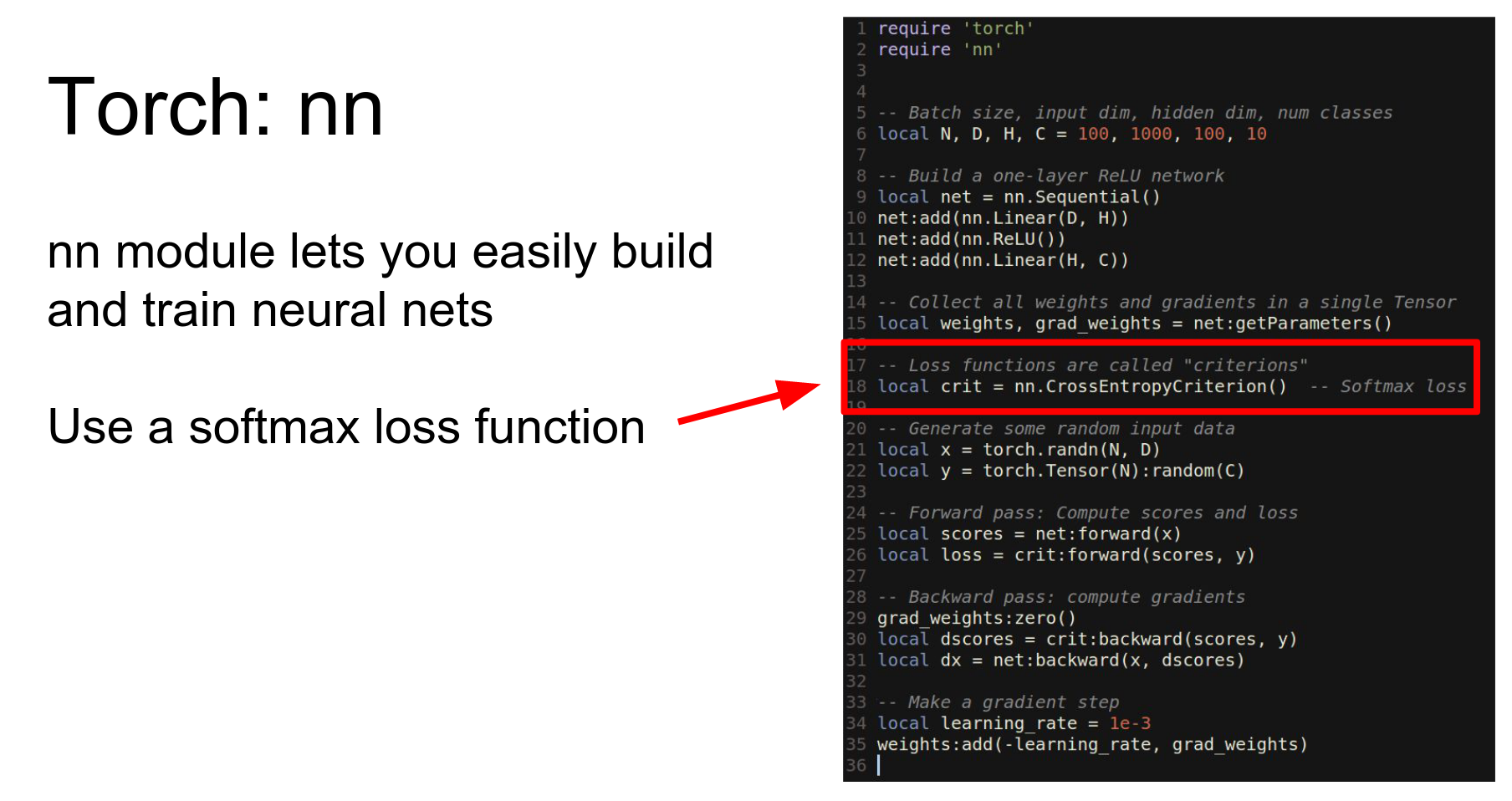
We have our loss function.

We get random data.

Run forward.

Run backward.

Make an update.

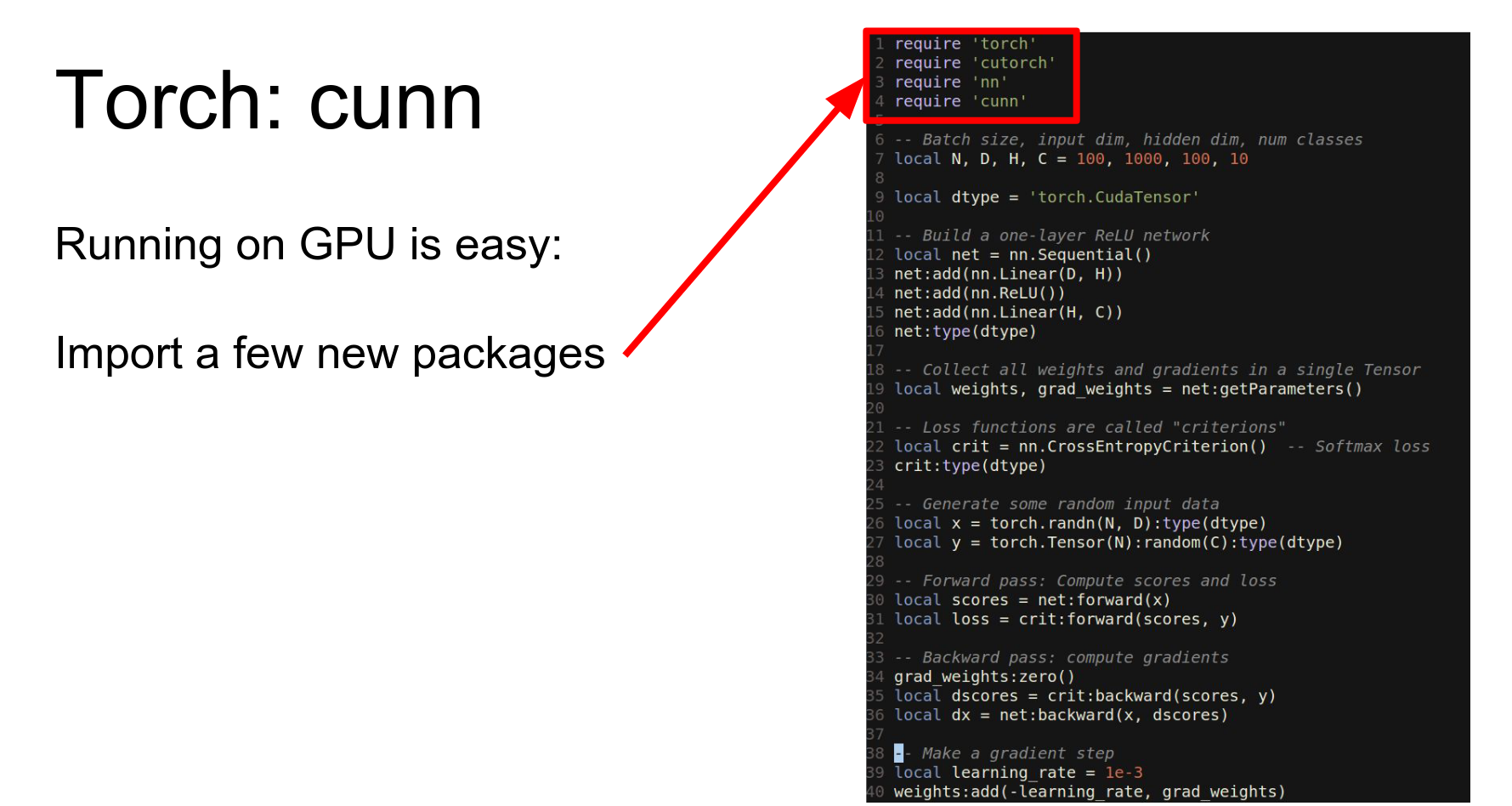
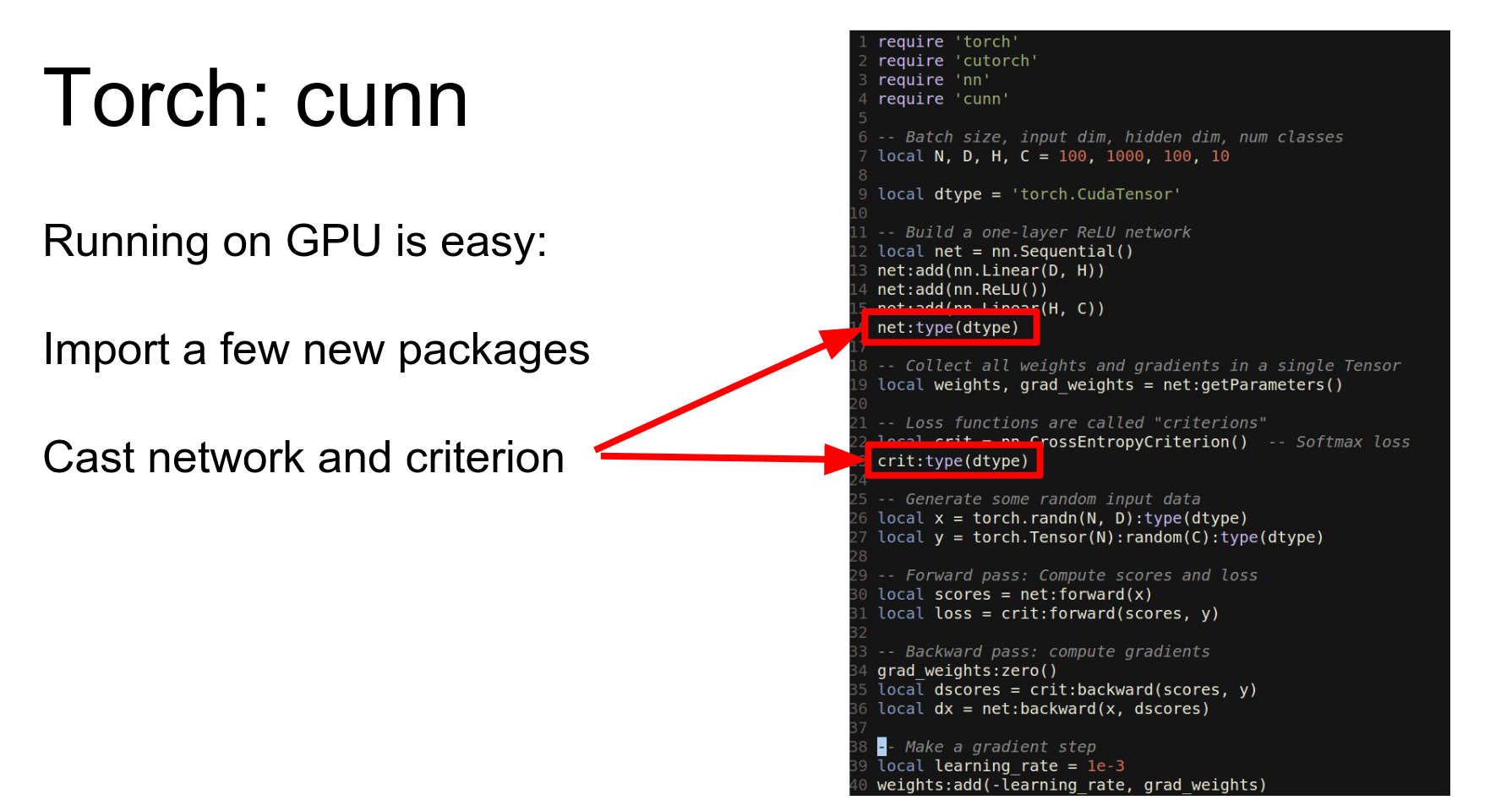
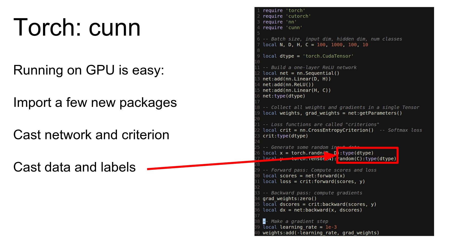
To run this on GPU, we import cutorch and cunn, cast our network and loss to CUDA, and cast our data to CUDA.

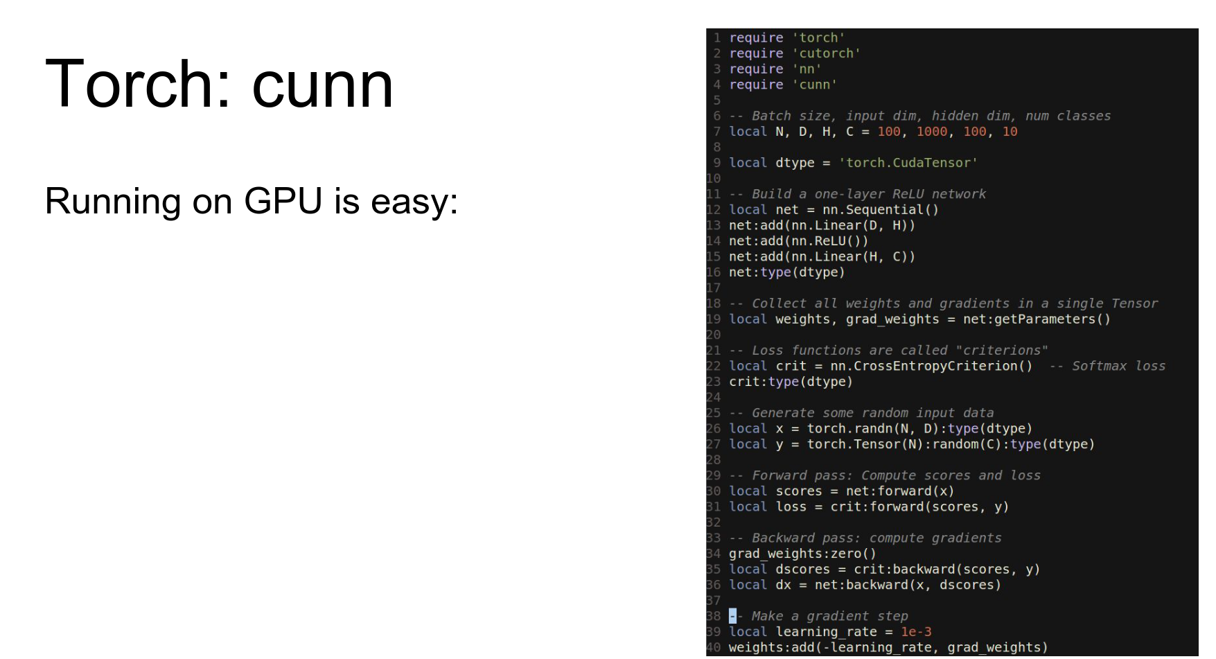
Then we just need to cast our network and our loss function to this other data type.

In 40 lines of code, we've written a fully connected network that trains on the GPU.

However, vanilla gradient descent is not great. We want to use Adam or RMSProp.

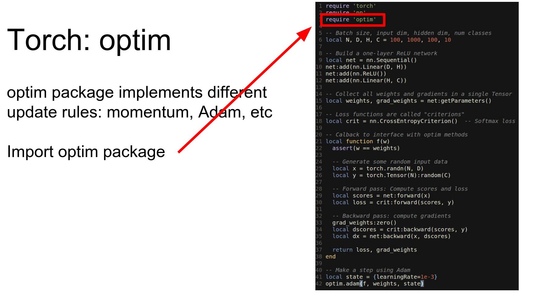
Torch gives us the optim package.

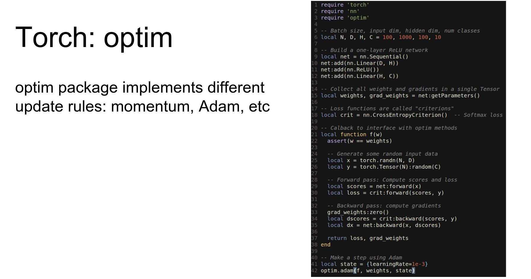
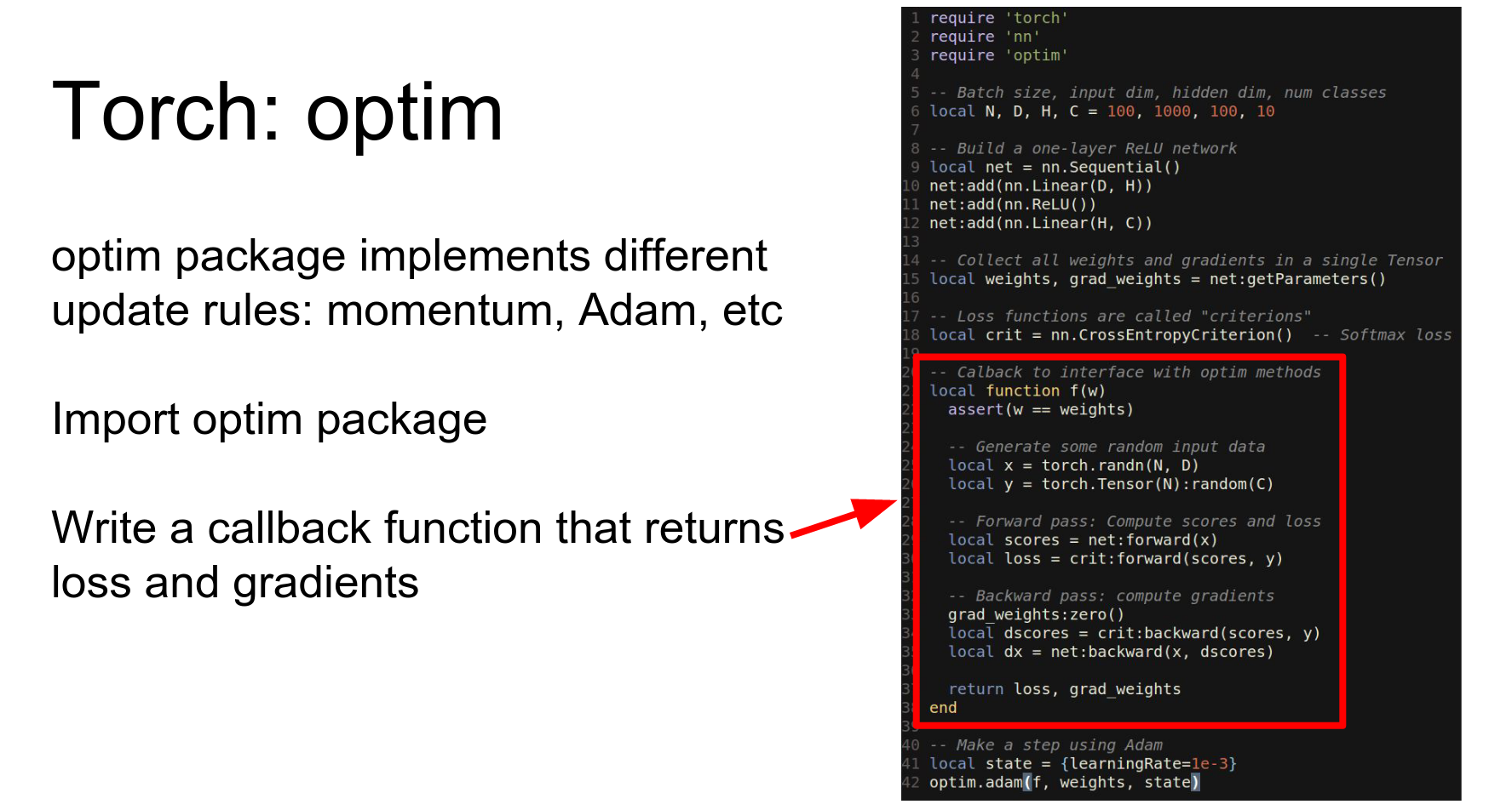
We define a callback function that runs the network forward and backward and returns the loss and gradients. Then we pass this callback to optim.adam.

In other words, what changes is that we actually need to define this callback function.

So before we were just calling forward and backward exclude explicitly ourselves instead we're going to define this callback function that will run the network forward and backward on data and then return the loss and the gradient.

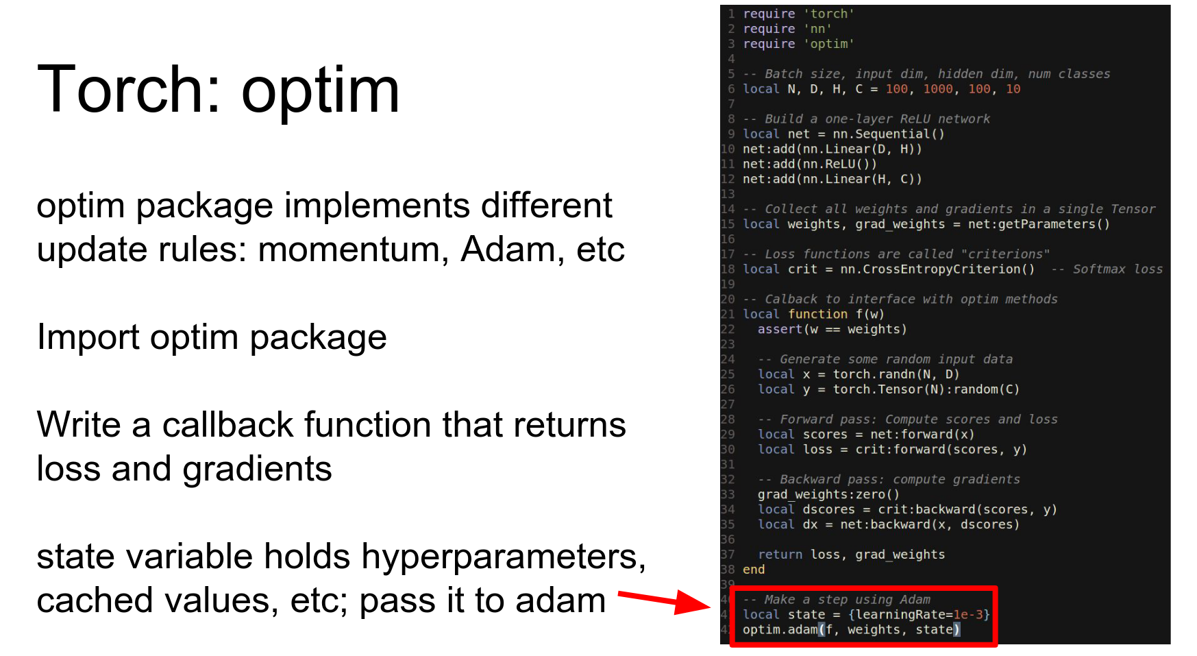
And now to make an update step on our network we'll actually pass this callback function to this Adam method from the optim package.

So this this is maybe a little bit awkward but we you now we can use any kind of update rule using just a couple lines of change from what we had before.

And again this is very easy to add to run on a GPU by just casting everything to CUDA.

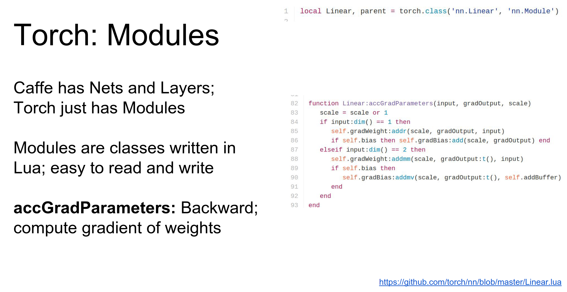
Caffe implements everything in terms of nets and layers. Caffe has this really hard distinction between a net and the layer.

In torch they don't we don't really draw this distinction everything is just a module. So the entire network is a module, and also each individual layer is a module.

Modules: In Torch, everything is a Module. The entire network is a module, and each layer is a module.

Modules are classes defined in Lua using the tensor API.

Here is the constructor for Linear. It sets up weight and bias tensors.

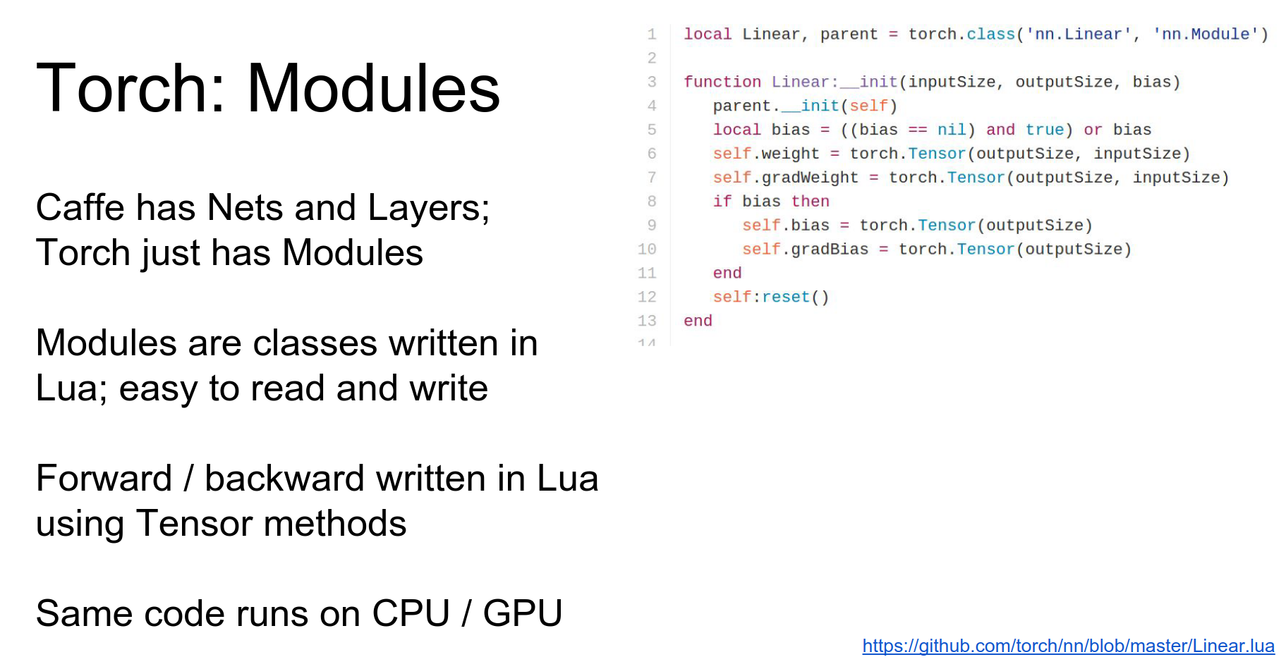
Modules implement updateOutput (forward) and updateGradInput (backward).

Here's the example of the update output for the fully connected layer.

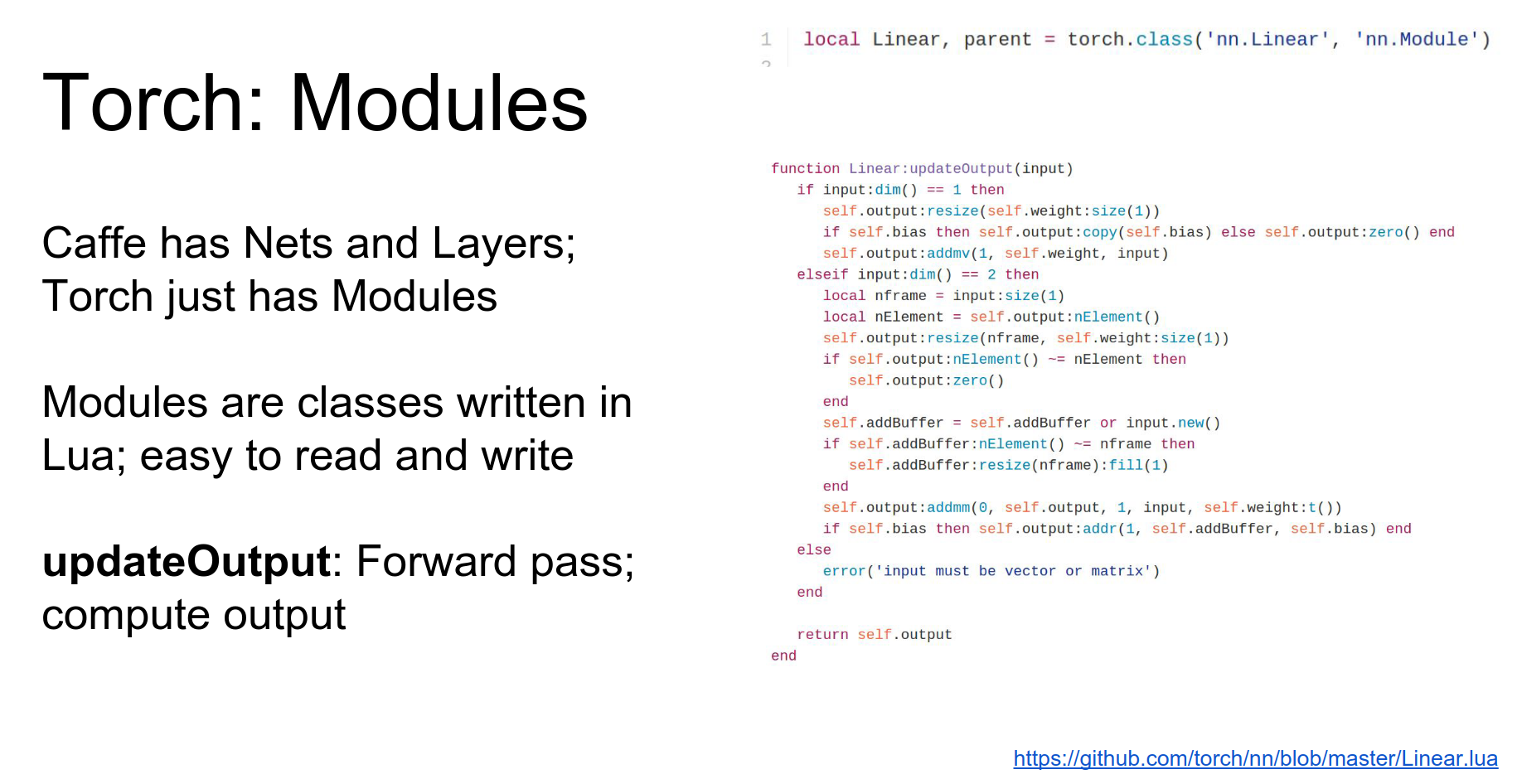
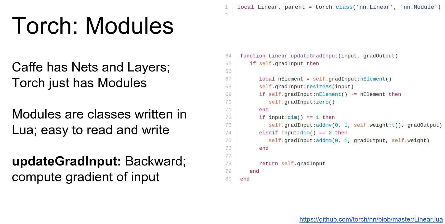
They also implement accGradParameters to compute gradients with respect to weights.

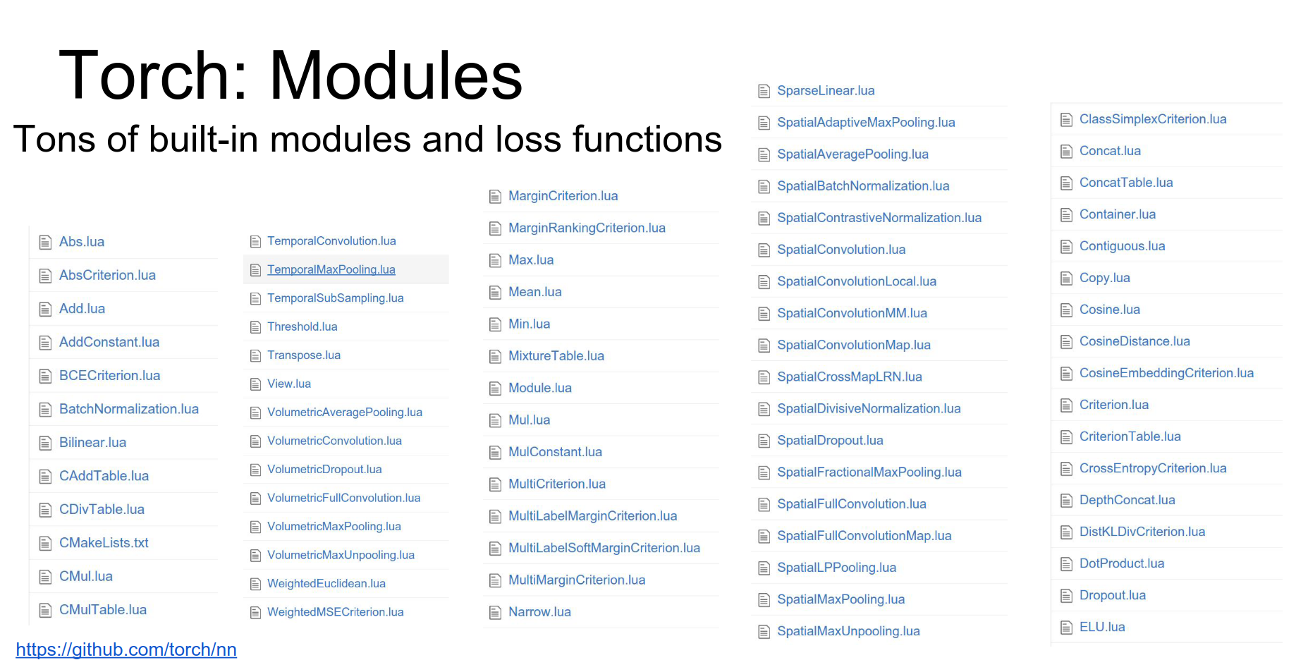
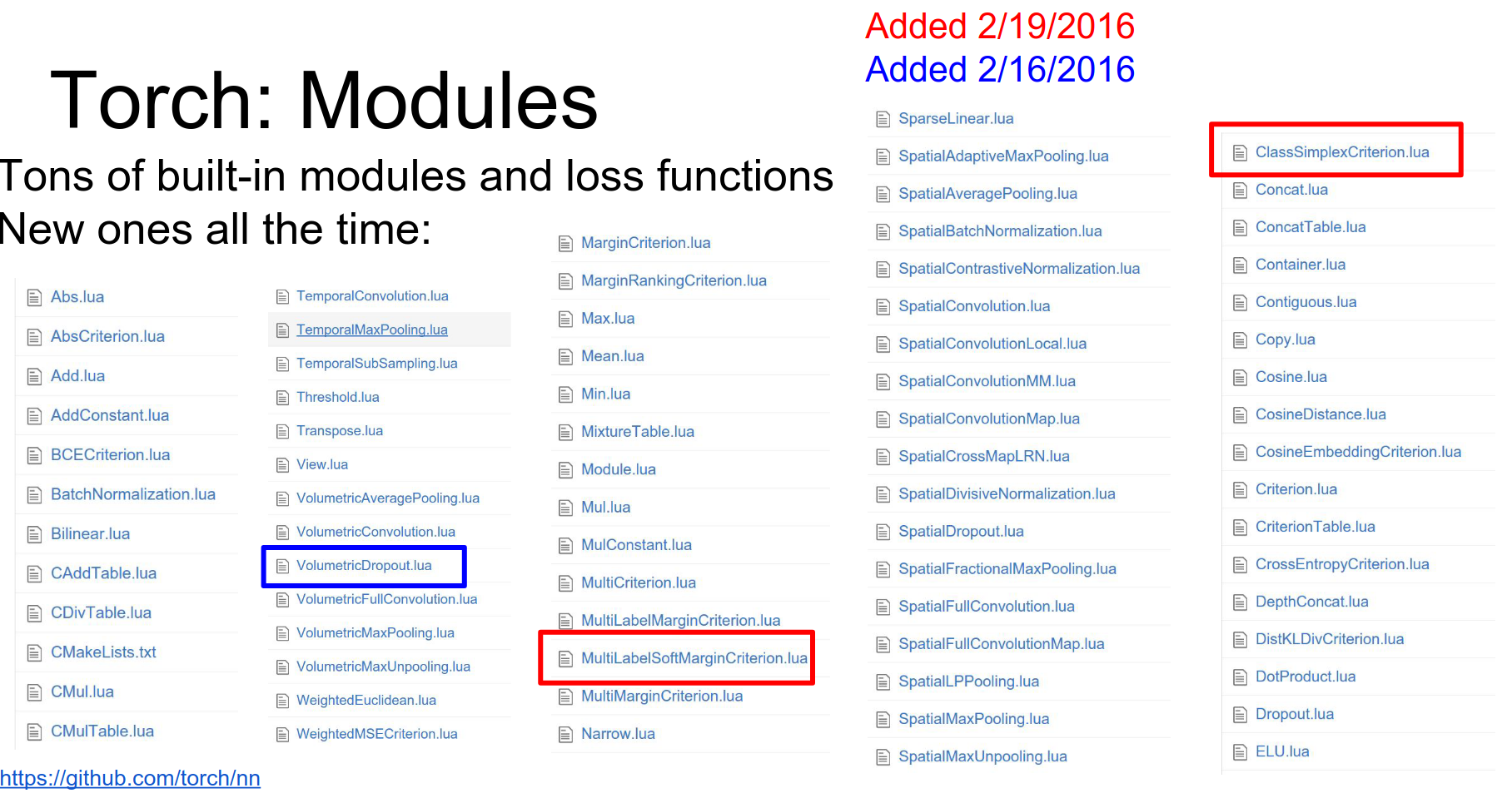
Torch has a ton of modules available. Check GitHub for the list.

These get updated a lot, so pay attention to the version you're using.

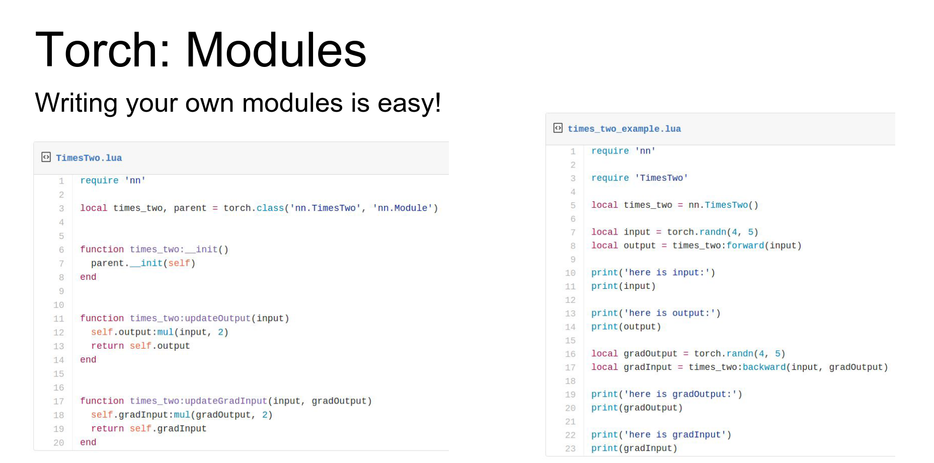
It is very easy to write your own modules. You just implement updateOutput and updateGradInput. You can do whatever arbitrary code you want inside (loops, stochastic things, etc.).

But of course using individual layers on their own isn't so useful we need to be able to stitch them together into larger networks.

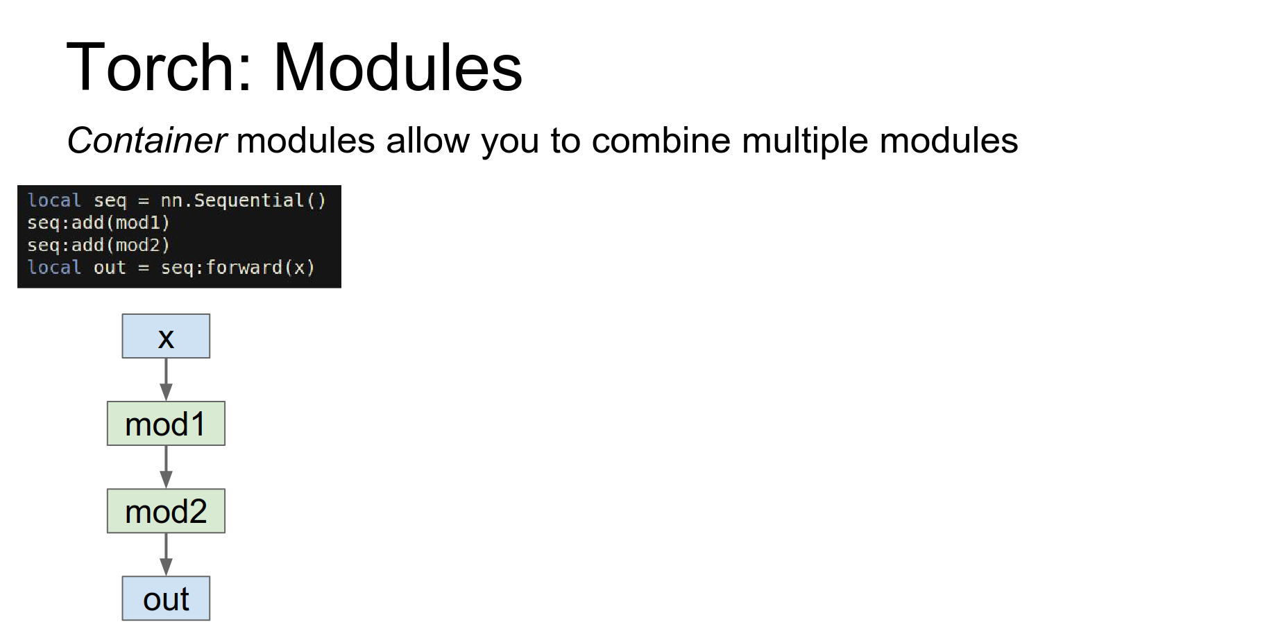
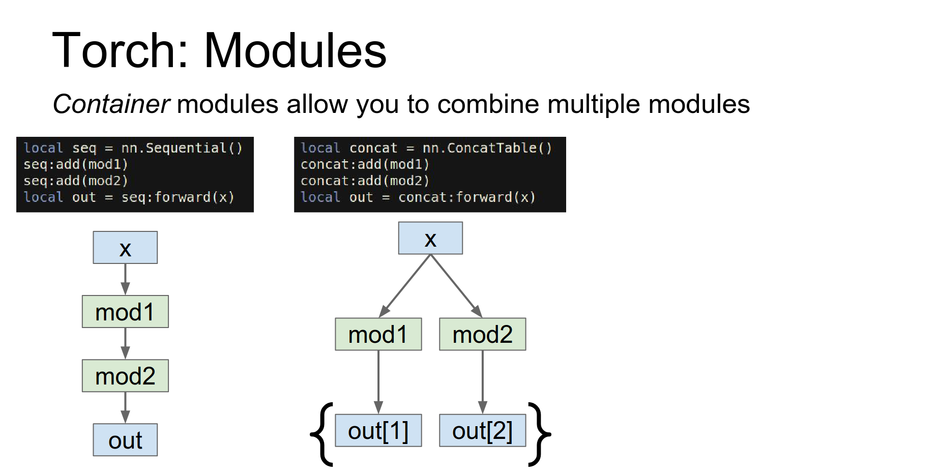
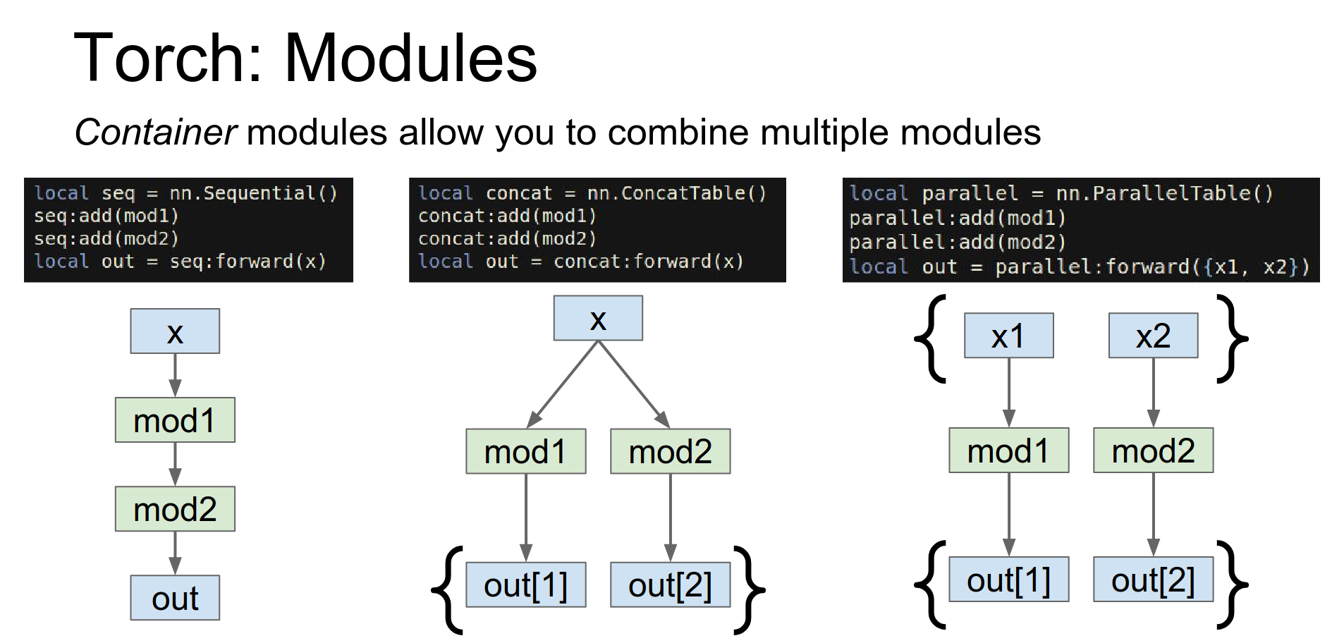
Containers: To stitch layers together, Torch uses containers.

• Sequential: A linear stack.

• ConcatTable: Apply different modules to the same input.

- ParallelTable: Apply different modules to a list of inputs.

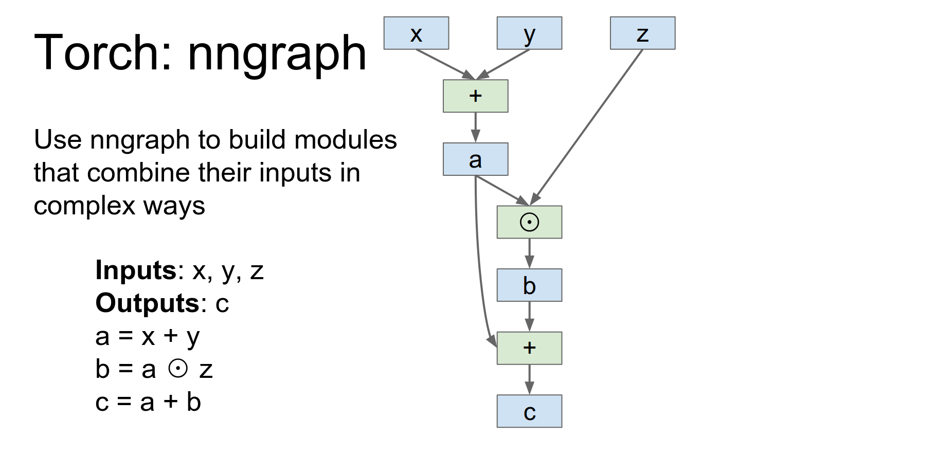
nngraph: For complicated topologies (like DAGs), Torch provides nngraph.

Those containers that I just told you should in theory make it possible to implement just about any topology you want.

Torch provides another package called nngraph, that lets you hook up things in more complicated topologies pretty easily.

So here's an example if we have three inputs and we want to produce one output, and we want to produce them with this pretty simple update rule.

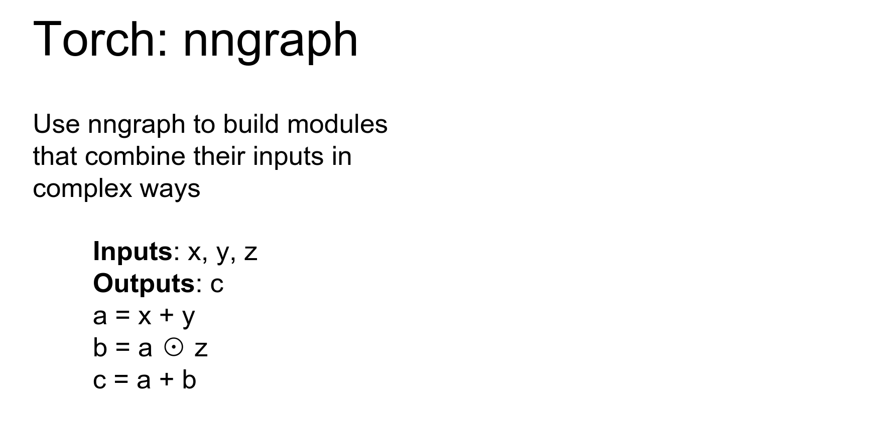
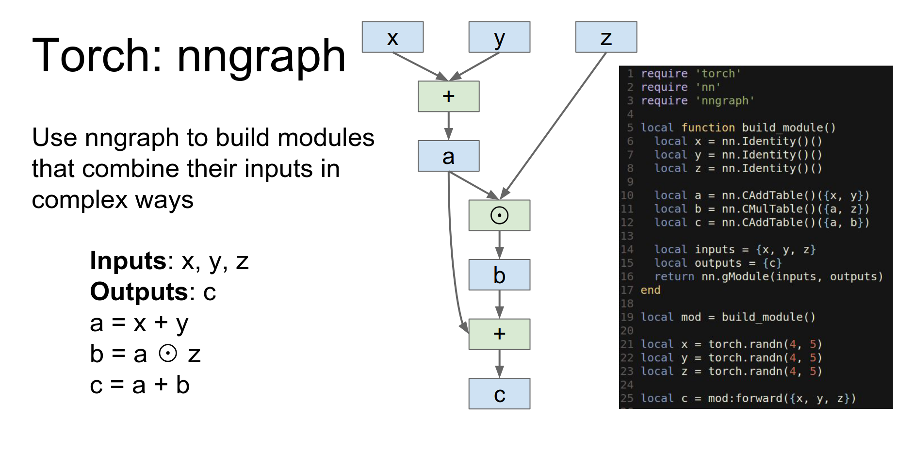
You define symbolic variables and build a graph. nn.gModule returns a module implementing this graph.

This function is going to build a module using nn graph and then return it.

So here we import the NNgraph package.

This is actually not a tensor this is defining a symbolic variable so this is saying that our our tensor object is going to receive x y and z as inputs and now here we're actually doing symbolic operations on those inputs.

So here we're saying that a we we want to have a point wise addition of x and y store that in a, we want to have point wise multiplication of a and Z and store that in B, and now point wise addition of a and B and store that in C.

These are not actual tensor objects these are now sort of symbolic references that are being used to build up this computational graph in the back end.

And now we can actually return a module here, where we say that our module will have inputs X,Y and Z and outputs C and this nn.gModule will actually give us an object conforming to the module API that implements this computation.

So then after we build the module we can construct concrete torch tensors and then feed them into the module that will actually compute the function.

Pre-trained Models: loadcaffe lets you load Caffe models (AlexNet, VGG) into Torch. There are also implementations for GoogLeNet and ResNet.

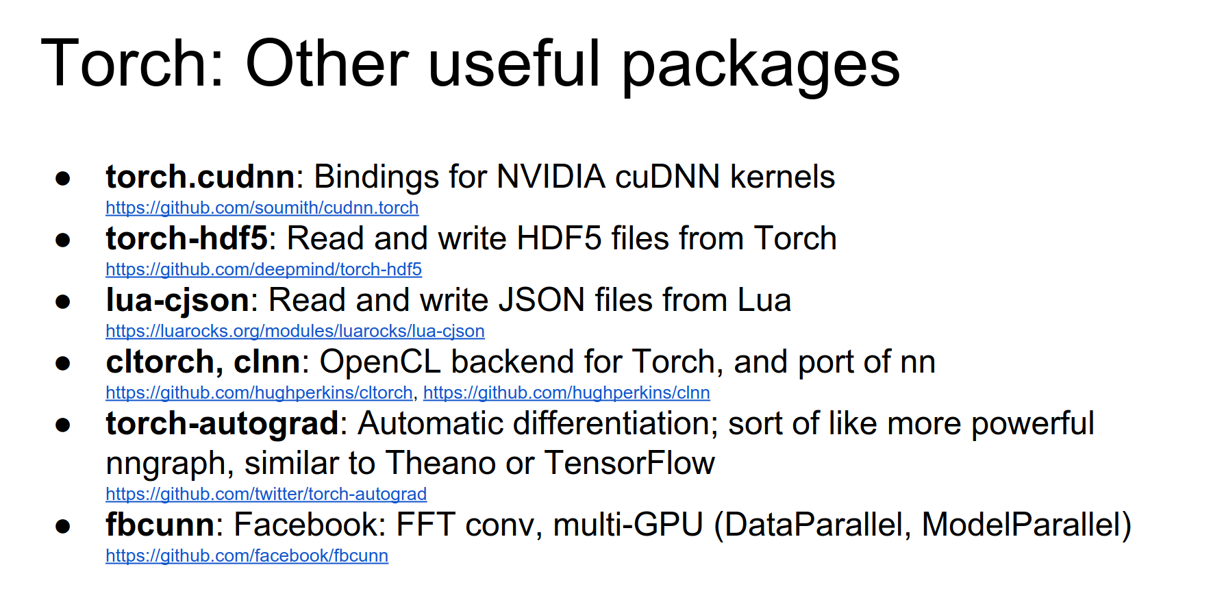
LuaRocks: Torch uses luarocks (like pip) to manage packages.

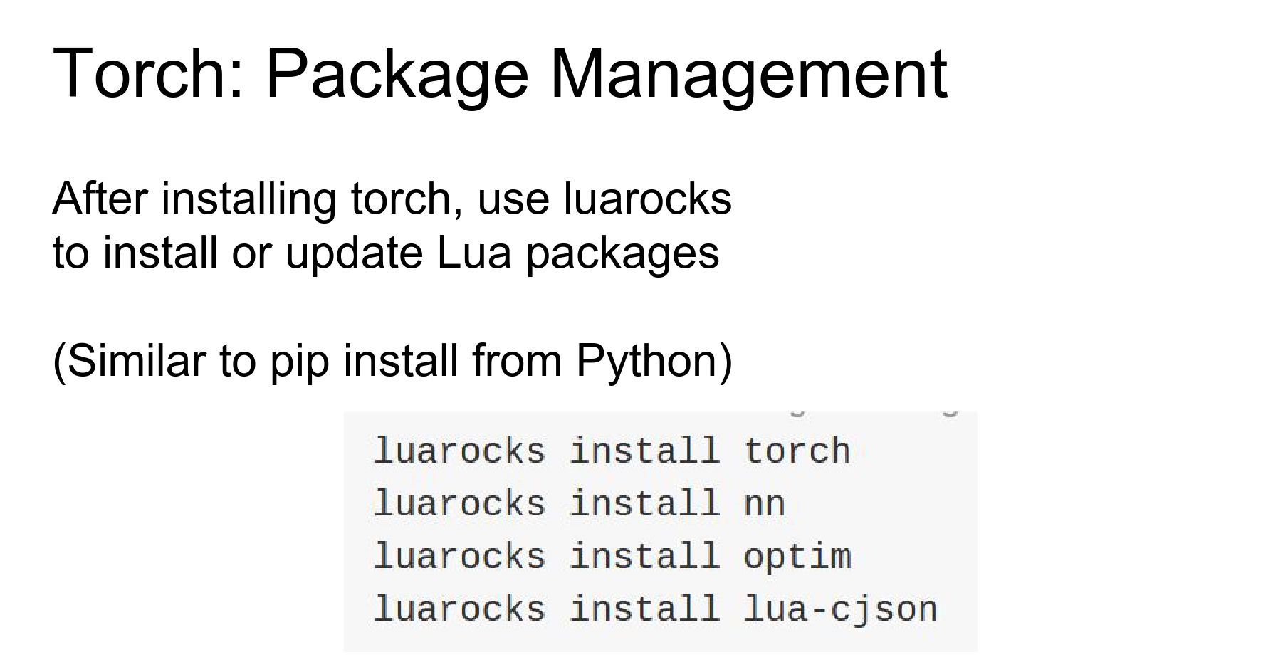
Useful packages: cudnn, hdf5, cjson, fbcunn.

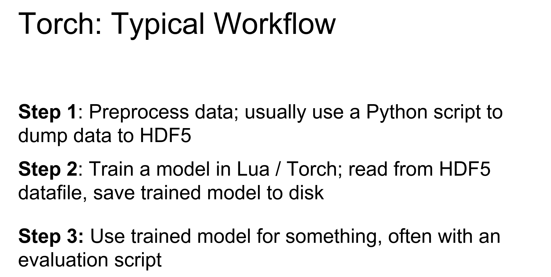
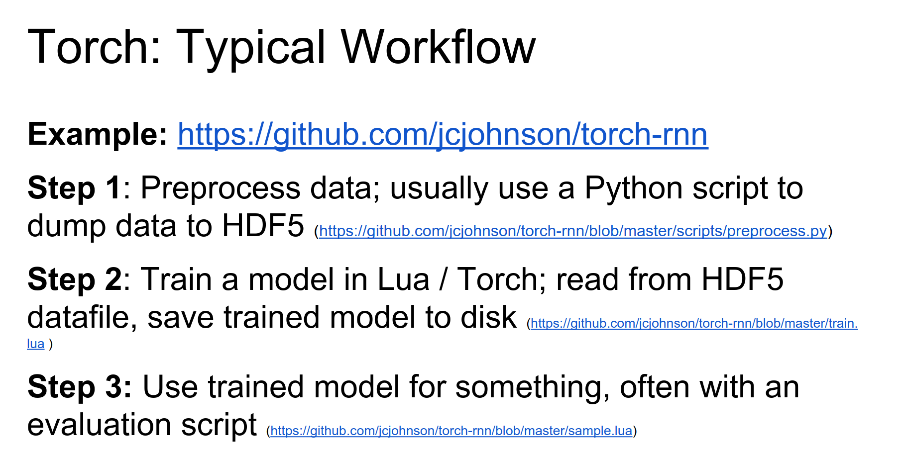
Typical Workflow:

1. Pre-processing script (Python) -> HDF5/JSON.
2. Train script (Lua) reads HDF5, trains model, saves checkpoints.
3. Evaluate script (Lua) loads checkpoints, generates outputs.

Case study on the page.

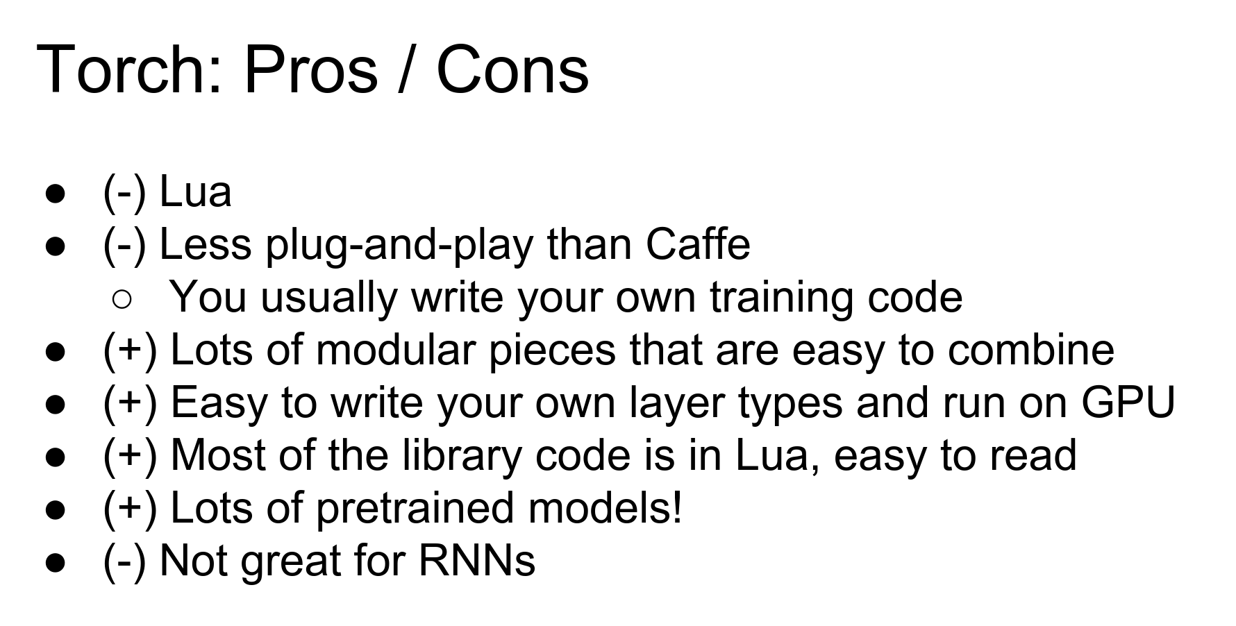
Torch Pros and Cons:

• Pros: Flexible, modular, easy to write custom layers, good pre-trained models. Lua is fast (JIT).
• Cons: Lua (unfamiliar to some), less plug-and-play than Caffe (you write code), RNNs can be tricky (sharing weights manually).

Performance: Lua is fast because of JIT compilation, similar to JavaScript engines. Python is slower for loops.

Theano

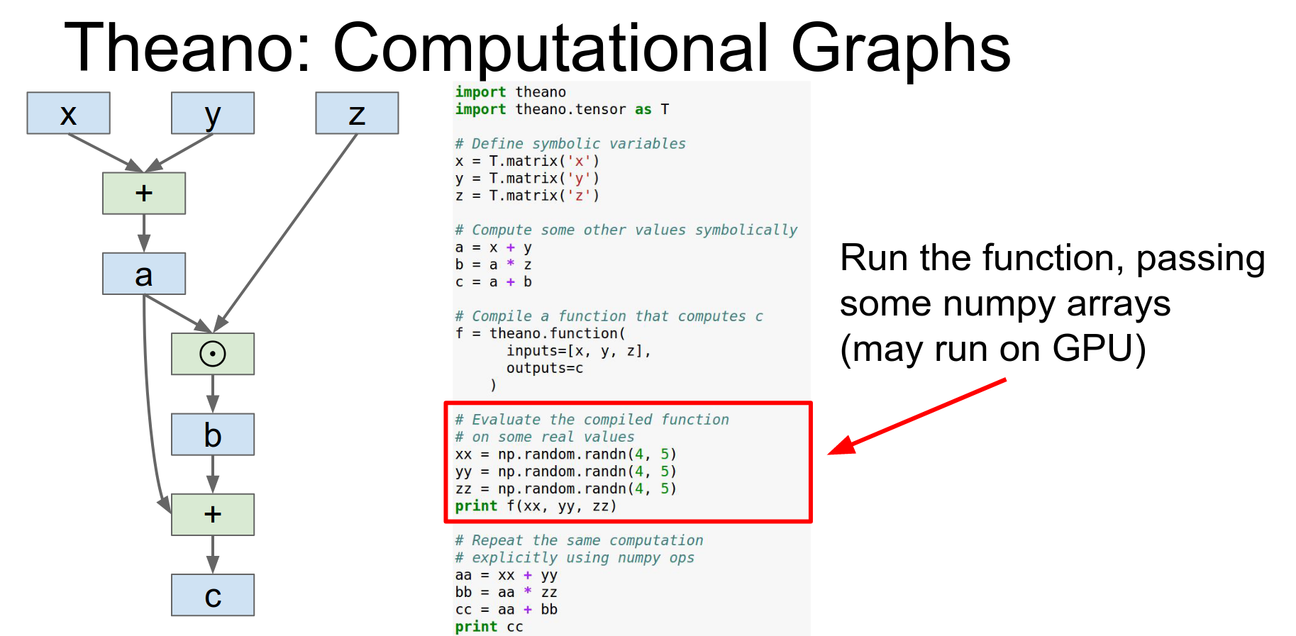
Theano is from Yoshua Bengio's group at the University of Montreal. It is all about computational graphs.

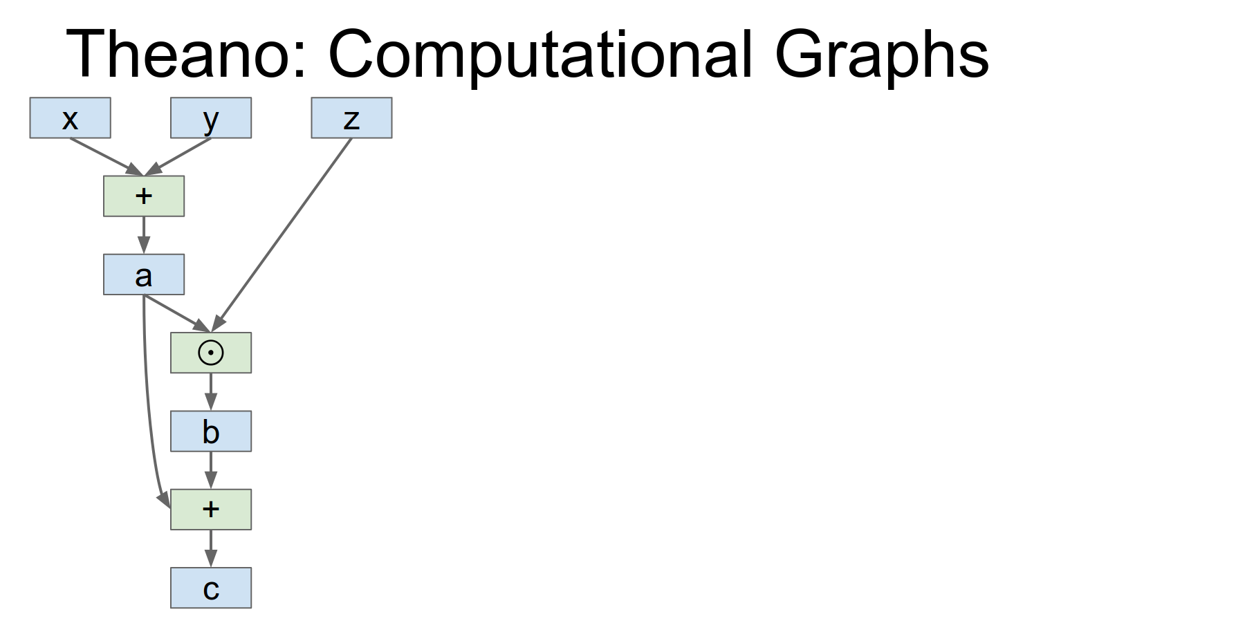
You define symbolic variables (x, y, z) and compute outputs symbolically.

We're importing Theano and the Theano tensor object.

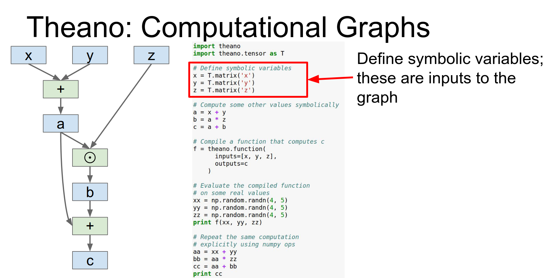
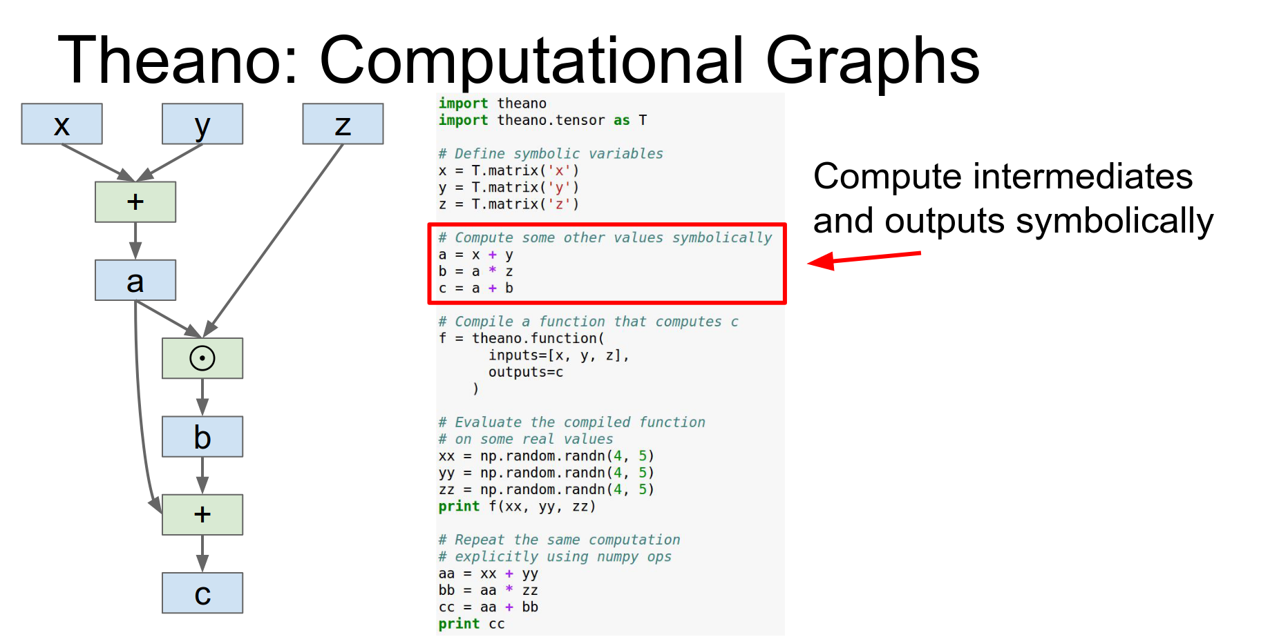
Then we can actually compute to these outputs symbolically so x,y&z are these symbolic things and we can compute a B and C just using these overload operators and that'll be building up this computational graph in the backend.

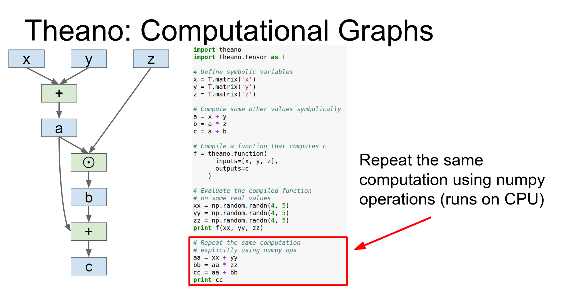
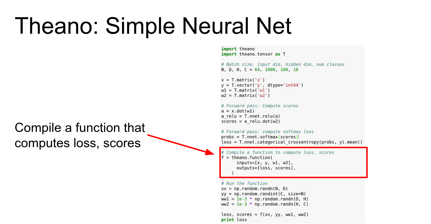
You compile a function using theano.function. This is where the magic happens: it optimizes the graph, derives gradients, and generates native code (possibly for GPU).

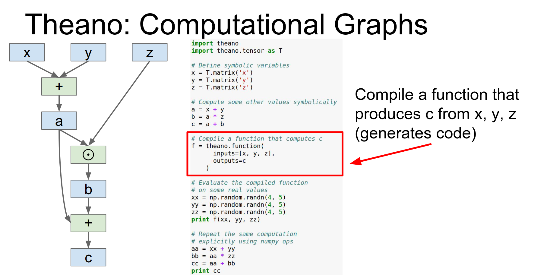
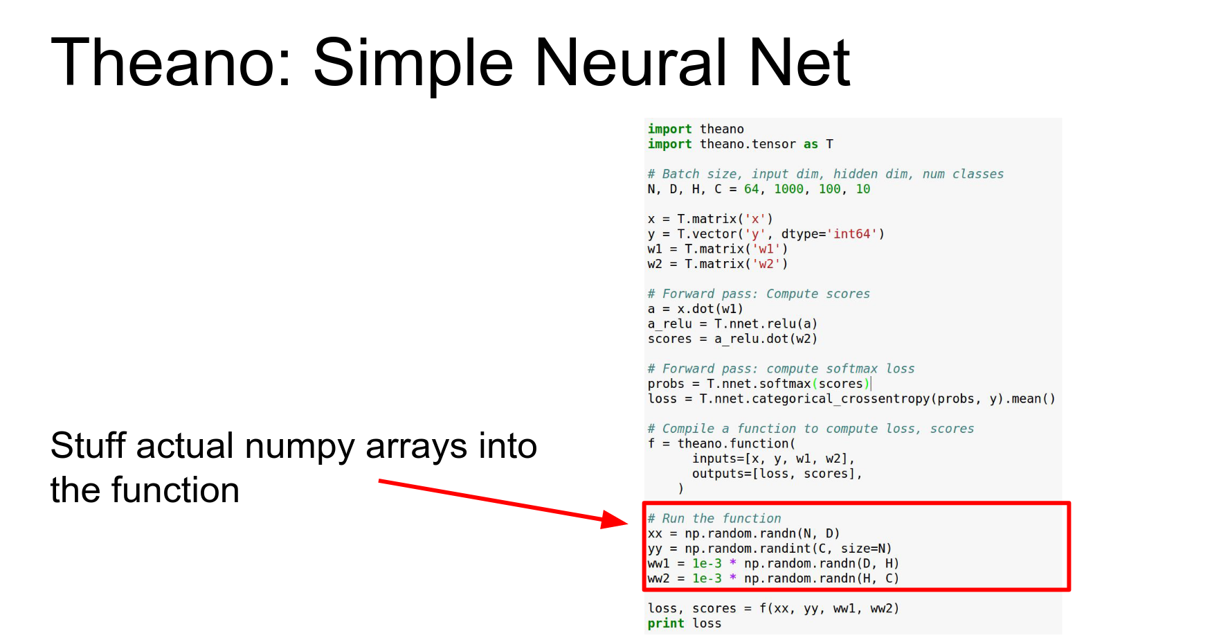
Then you run it on numpy arrays.

Neural Nets in Theano:

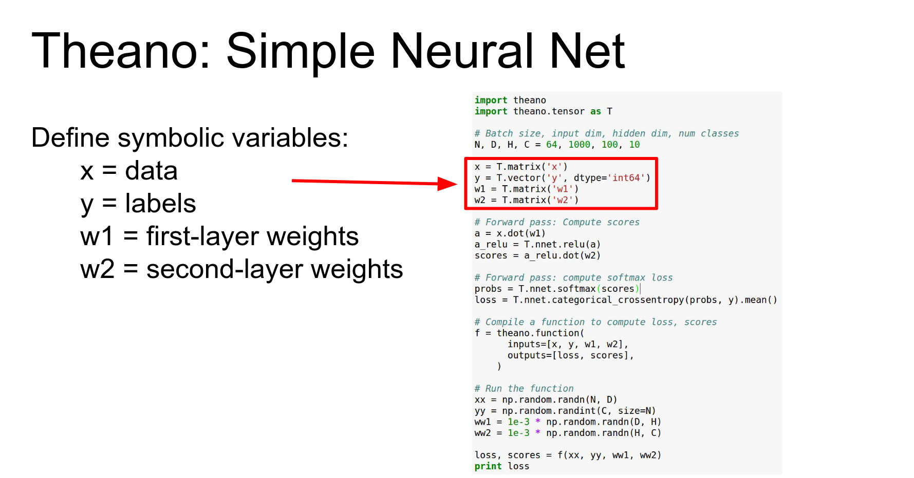
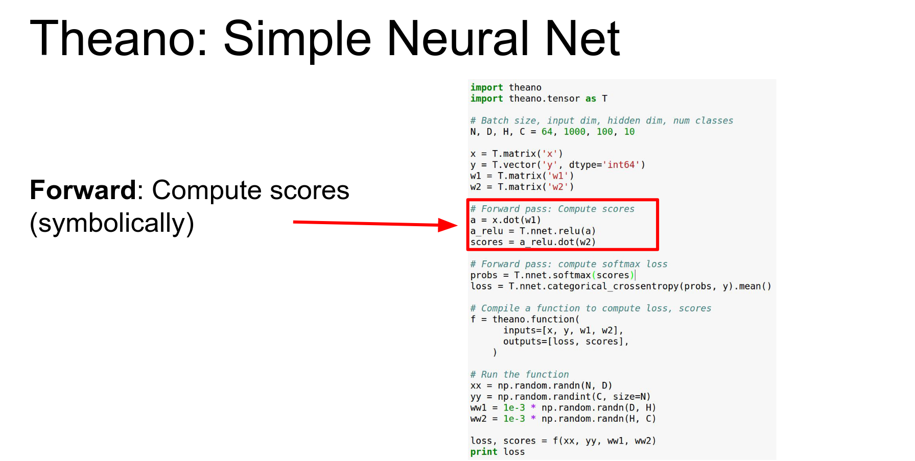
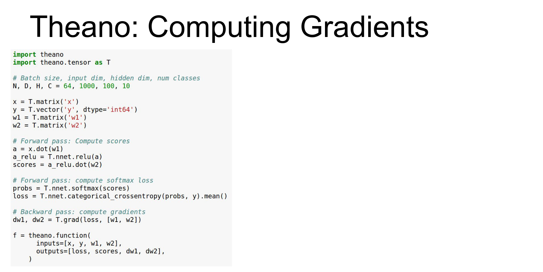
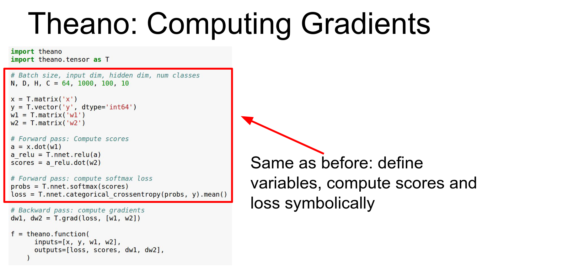
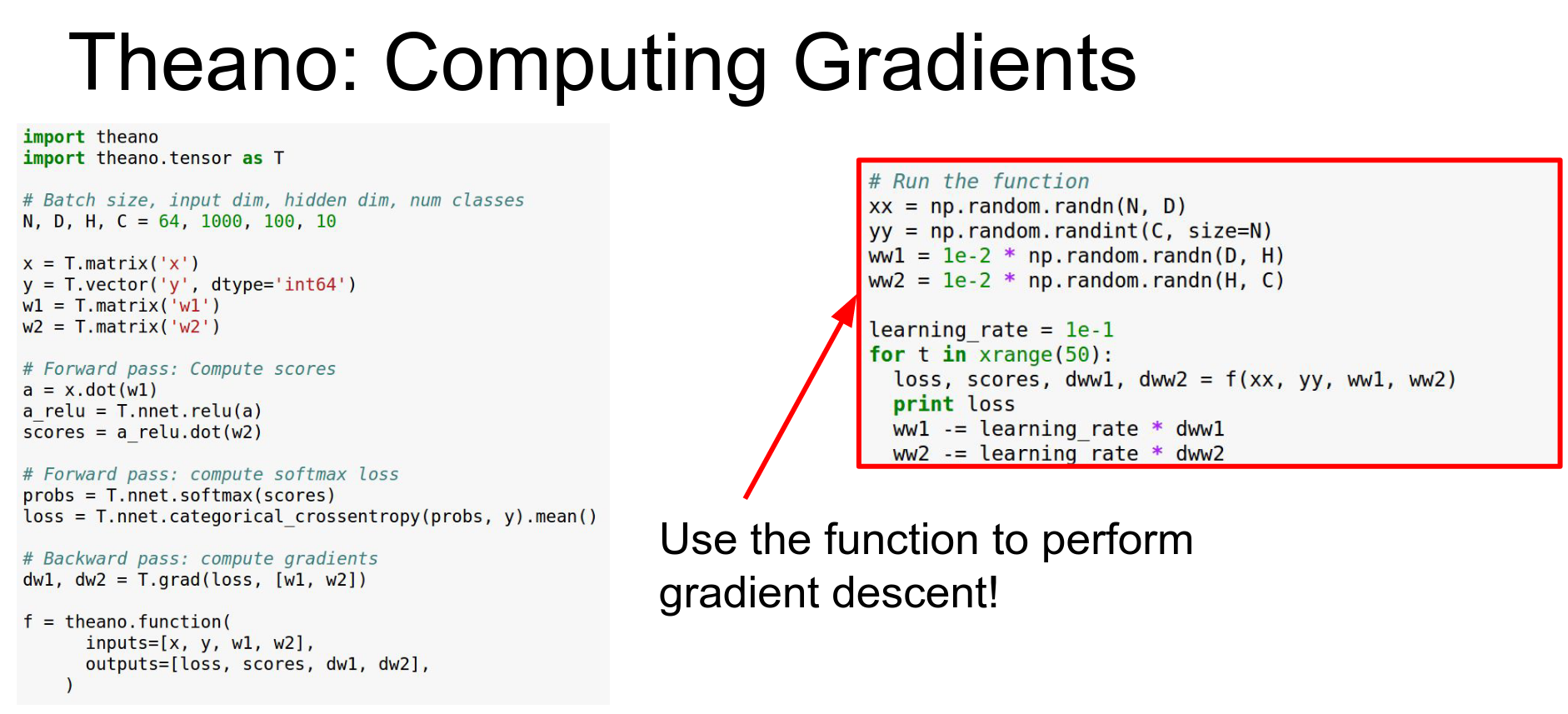
Define symbolic variables for inputs, labels, and weights. Here's an example of a simple two-layer ReLU in Theano.

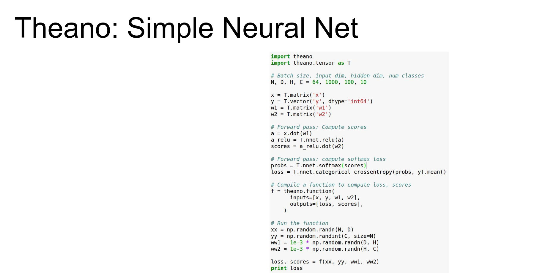
The idea is the same, that we're going to declare our inputs, but now instead of just x, y&z we have our inputs in X our labels in Y which are a vector and our two weight matrices W1 and W2.

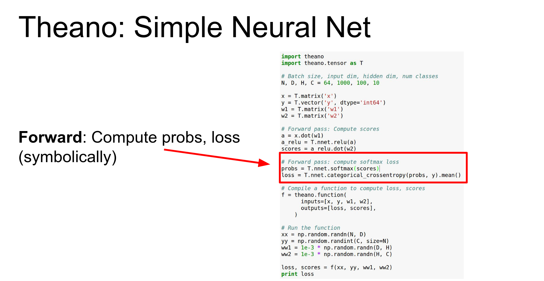
Define forward pass symbolically.

Compute loss symbolically.

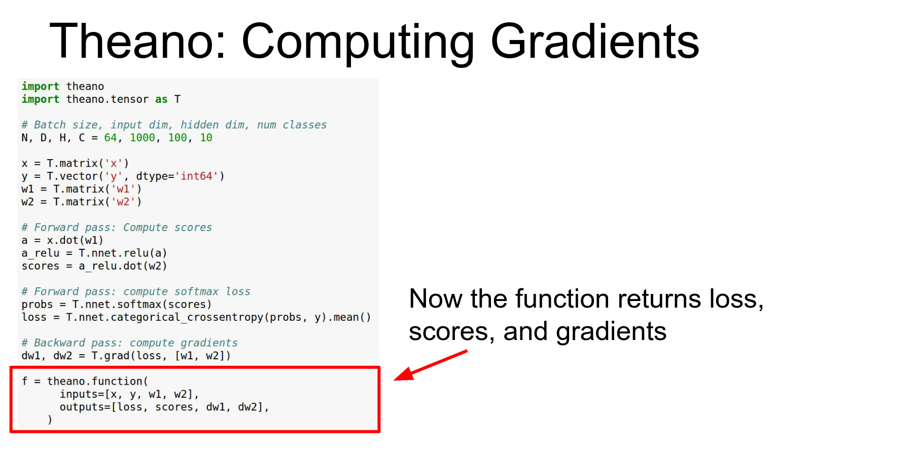
Compile function. As outputs that will return the loss in a scalar and our classification scores and a vector.

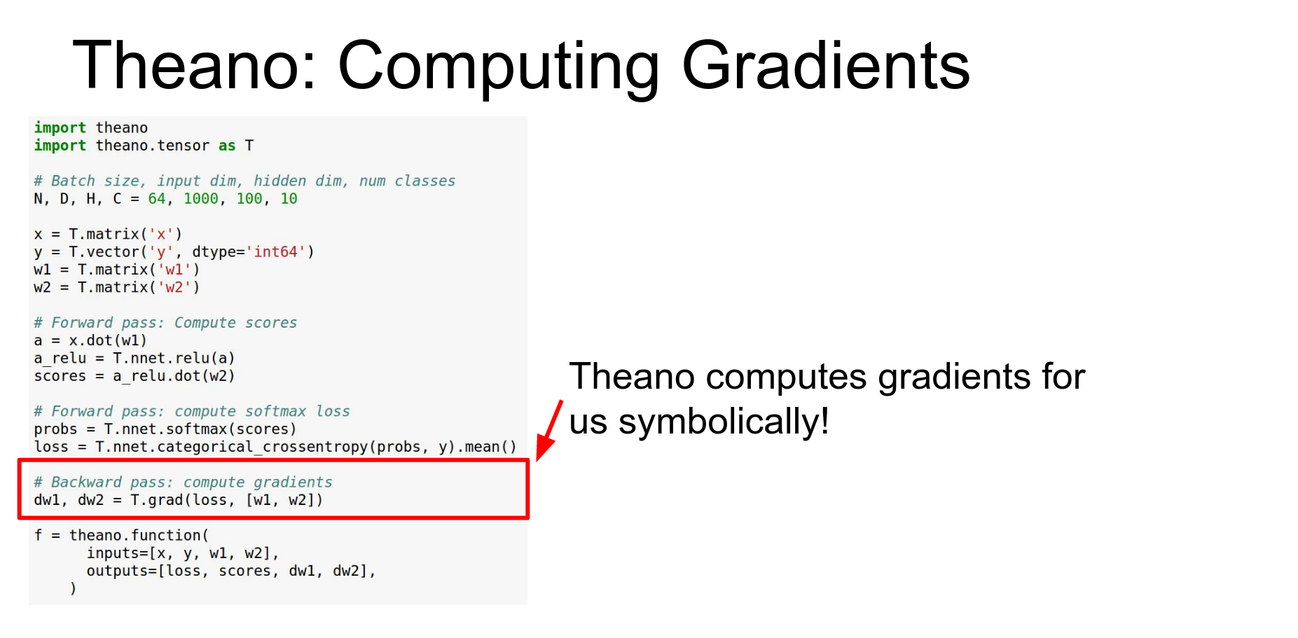
Gradients: Theano can do symbolic differentiation. T.grad computes gradients of the loss with respect to weights.

Here we just need to add a couple lines of code to do that.

This is the same as before we're defining our symbolic variables for our inputs and our weights.

Now the difference is that we actually can do symbolic differentiation here so this DW1 + DW2 we're telling Theano that we want those to be the gradients of the loss with respect to those other symbolic variables W1 and W2.

Theano just lets you take arbitrary gradients of any part of the graph with respect to any other part of the graph and now introduce introduce those as new symbolic variables in the graph.

Here in this case we're just going to return those gradients as outputs.

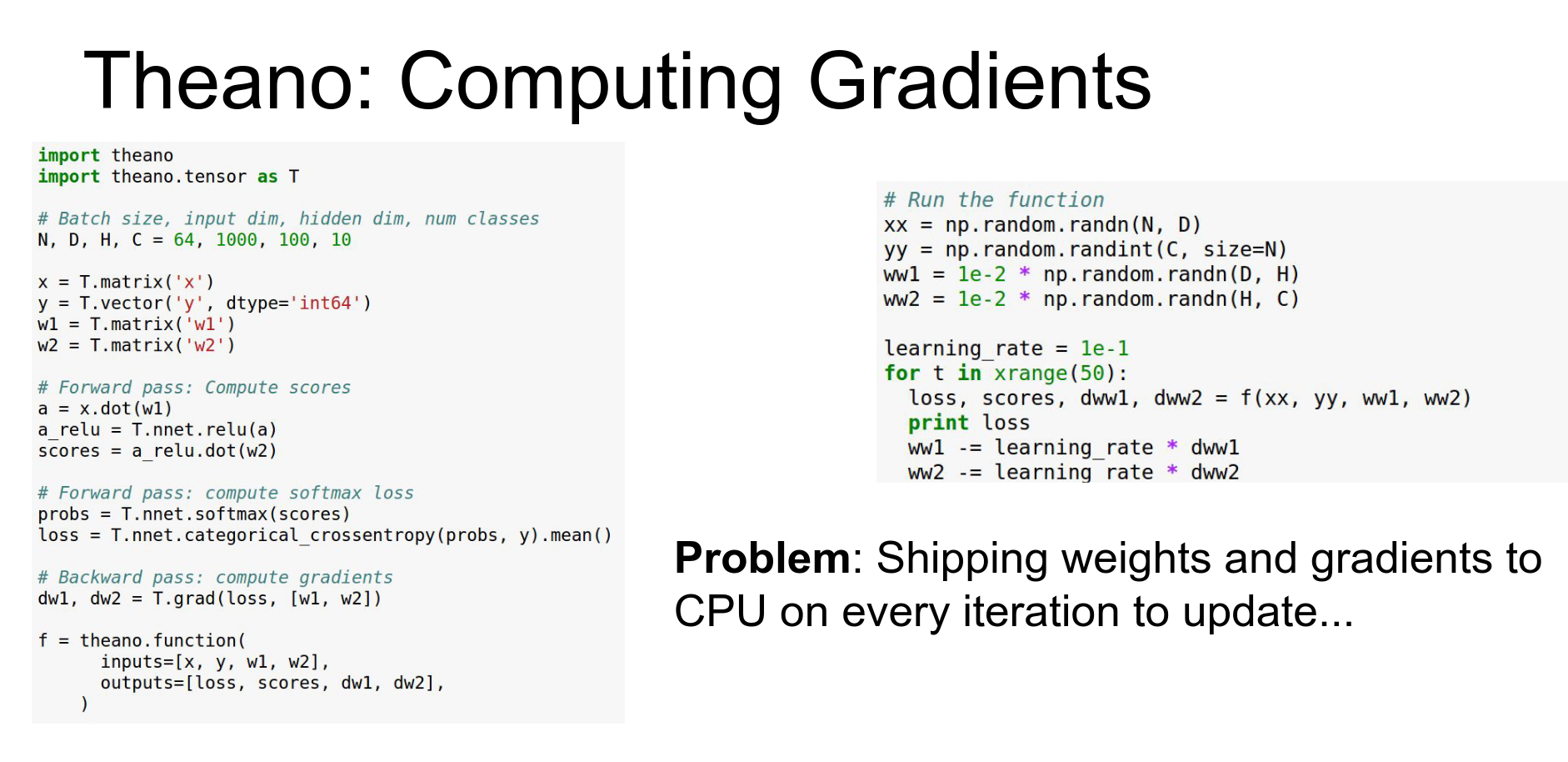
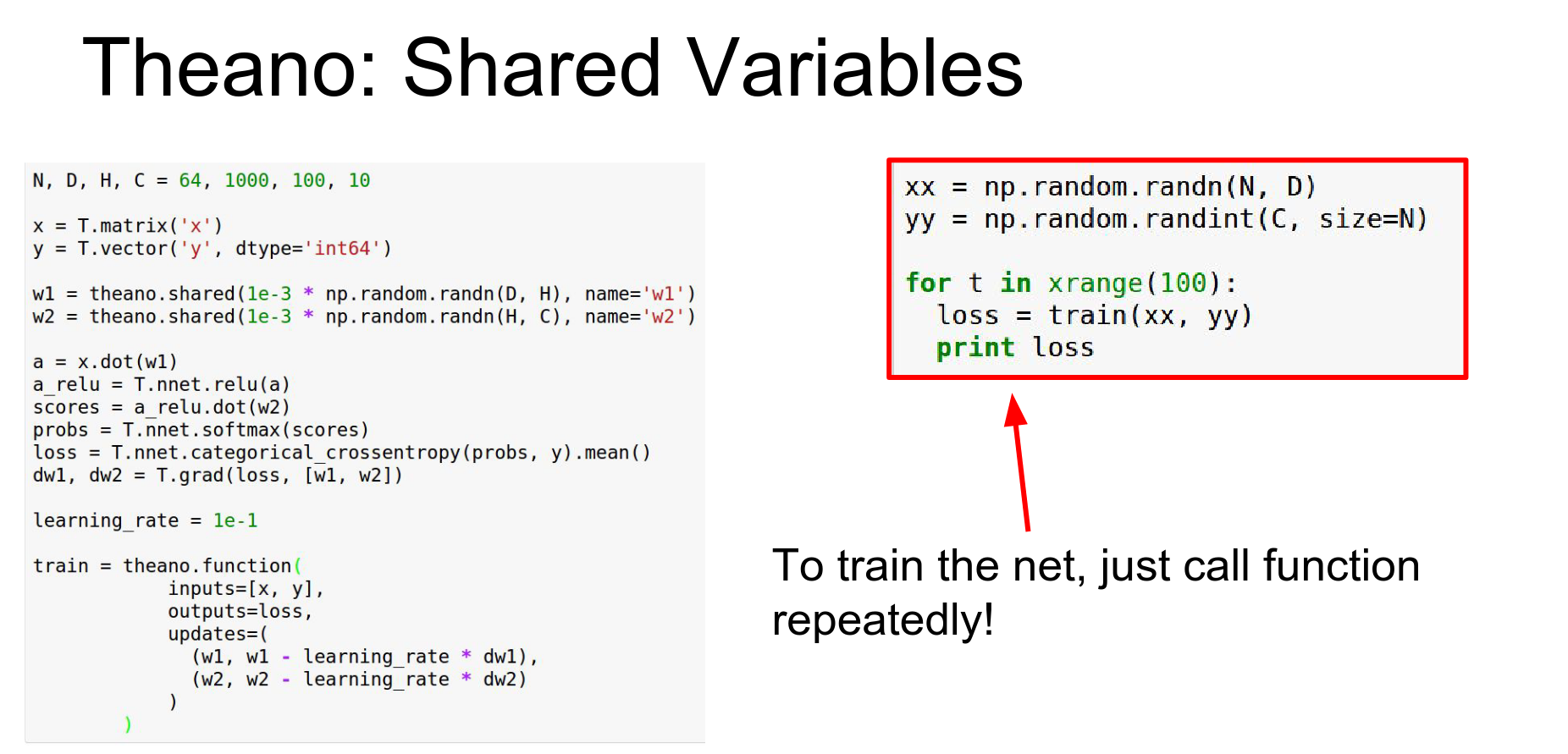
You can implement gradient descent by getting gradients and updating weights in a loop (in Python).

Problem: Updating weights in Python incurs CPU-GPU communication overhead.

Every time we call this f function and we get back these gradients that's copying the gradients from the GPU back to the CPU and that can be an expensive operation

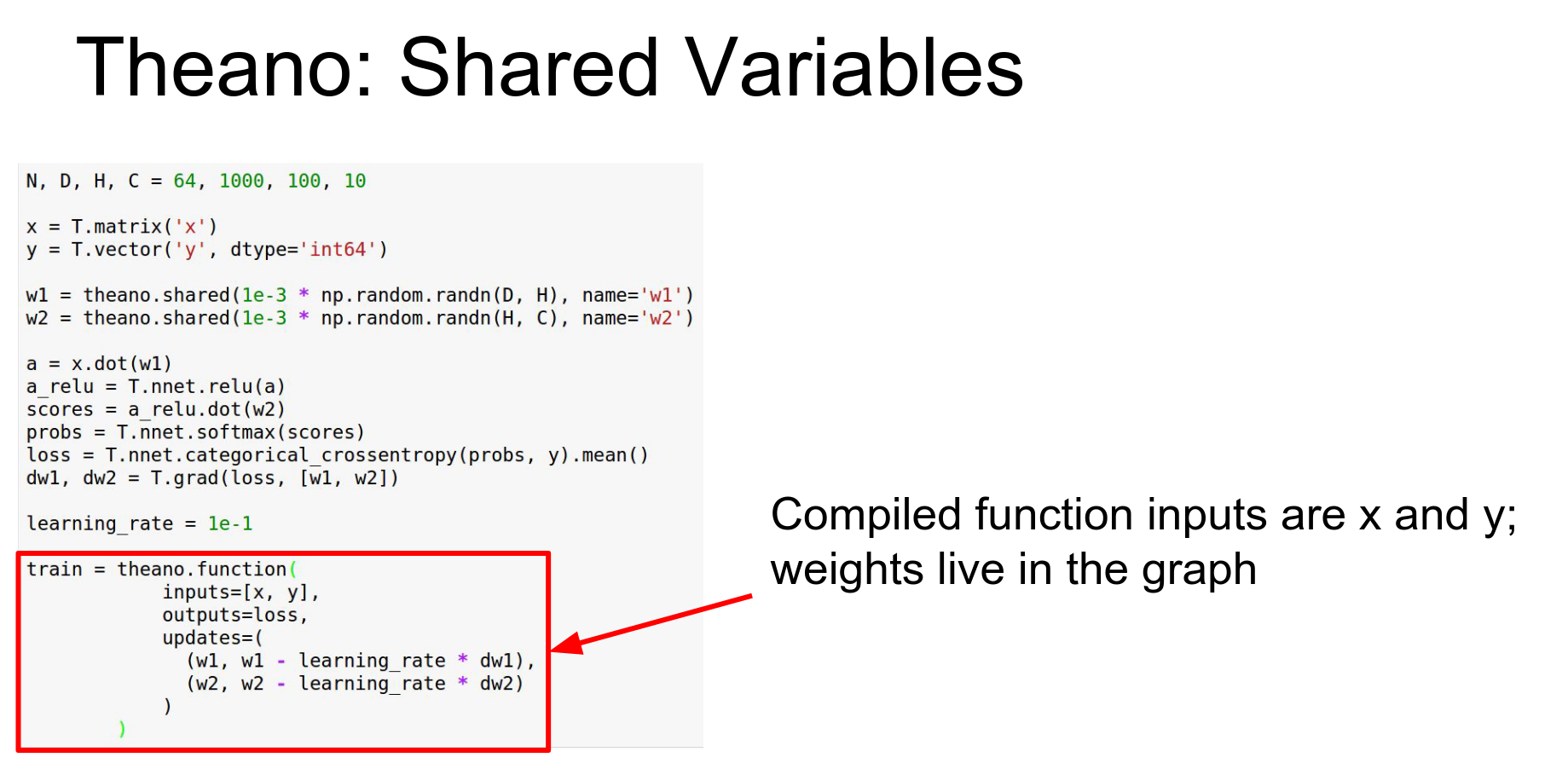
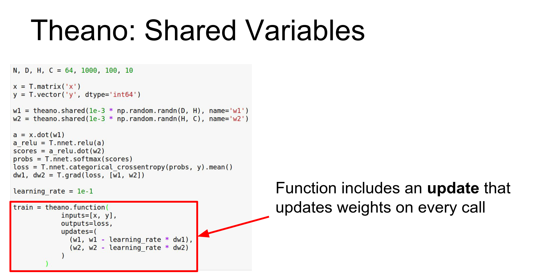
Shared Variables: To fix this, use Shared Variables. These live inside the computational graph and persist.

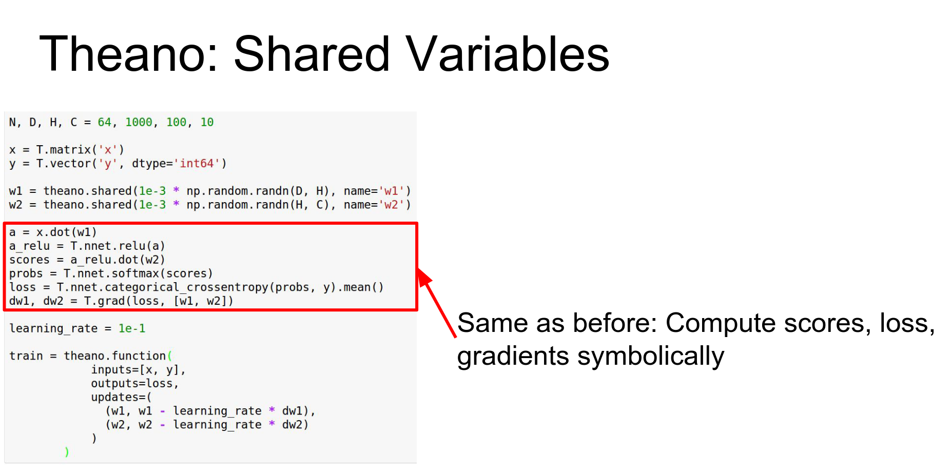
You define updates in the theano.function call. This updates the shared variables directly on the GPU every time the function is called.

We include this update.

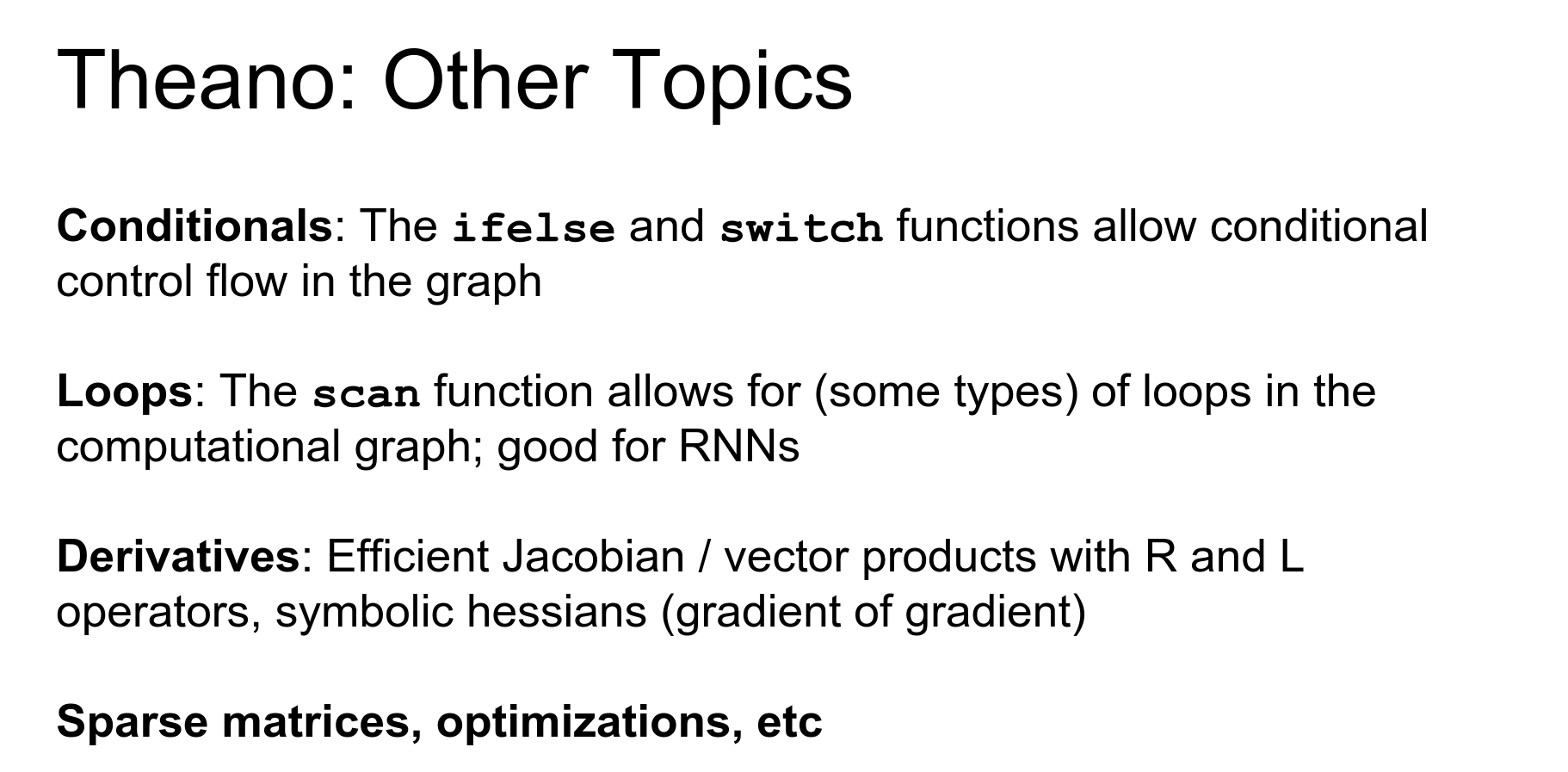
Advanced Theano: Conditionals, Loops (scan), Jacobians, R-operators.

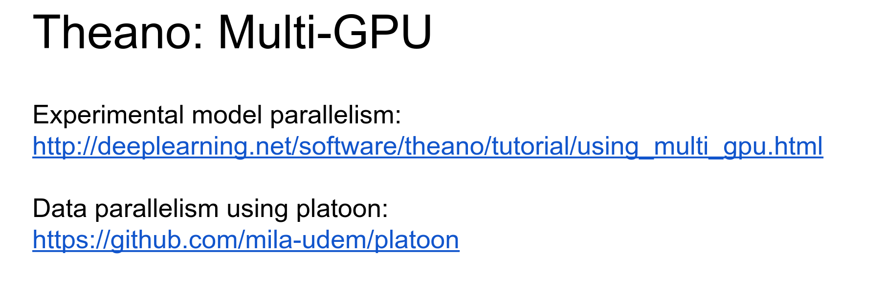
Theano has multi-GPU support (experimental).

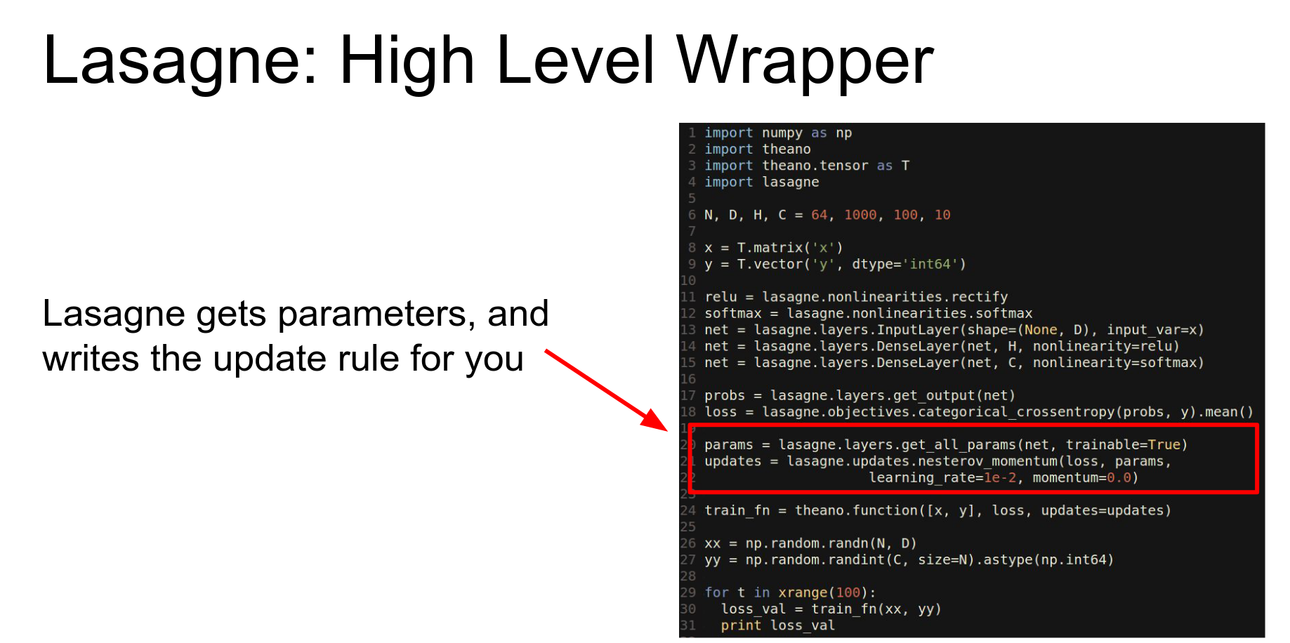
Lasagne: A high-level wrapper around Theano. It abstracts away the details.

Sweet abstraction.

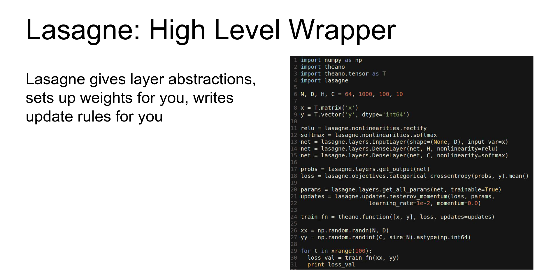
So again we're sort of defining symbolic matrices.

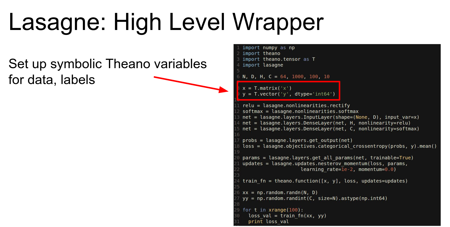
And Lasagne now has these layer functions that will automatically set up the shared variables.

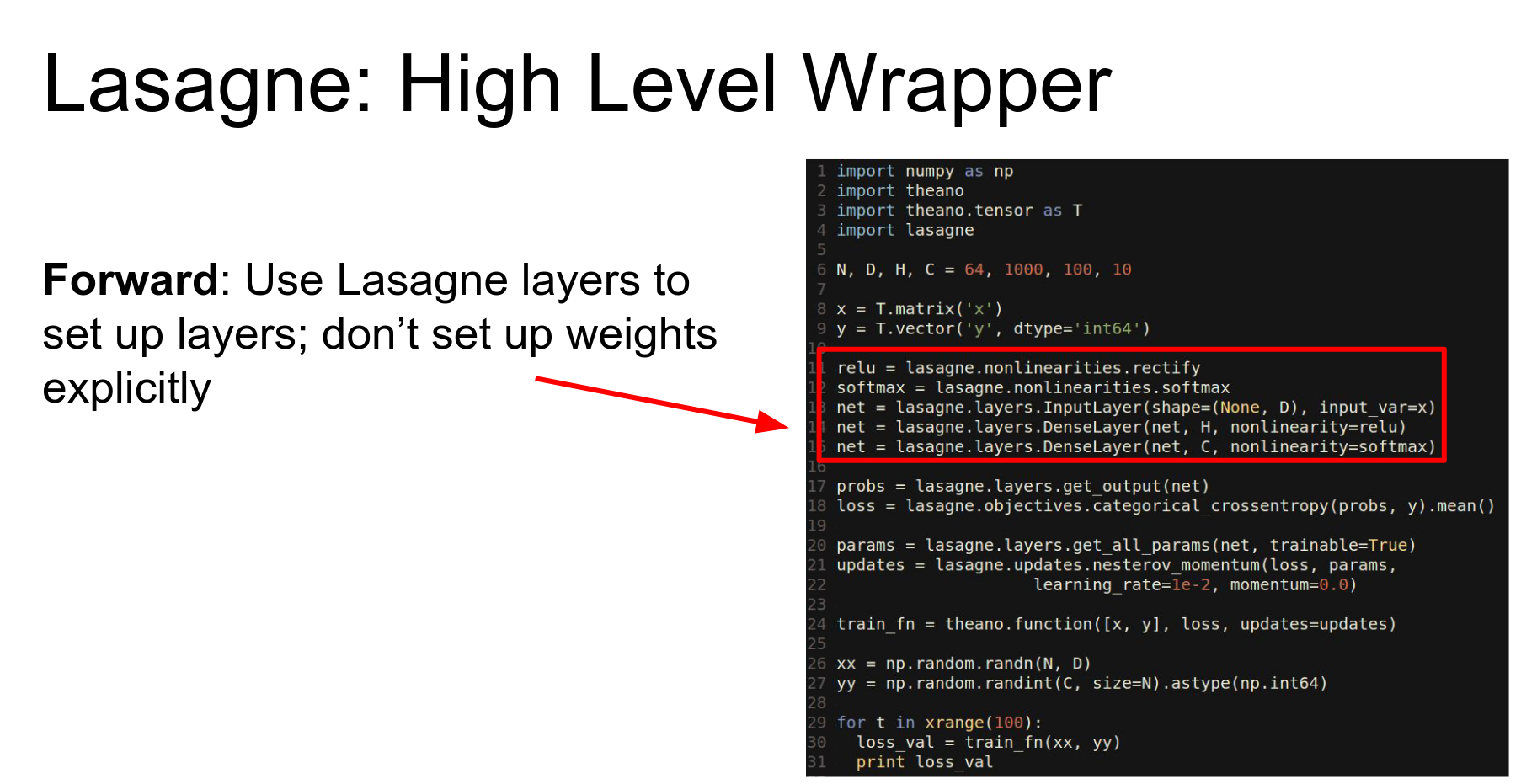
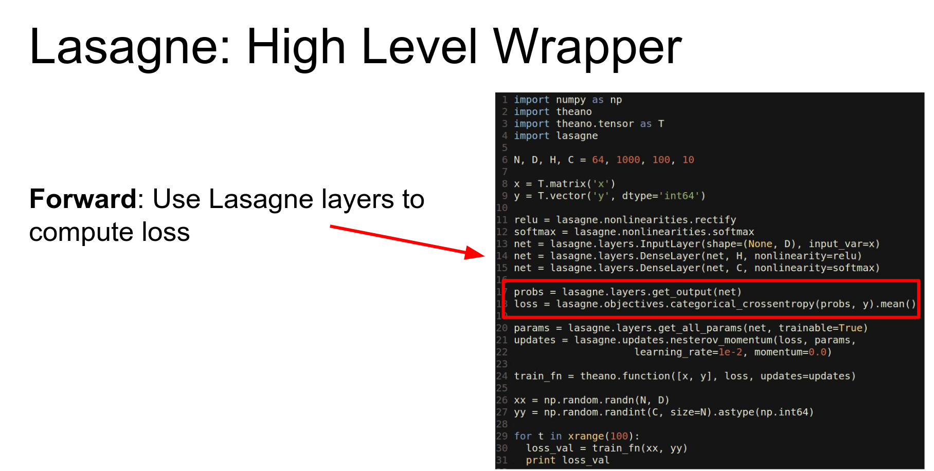
We can compute the probability in the loss using these convenient things from the Lasagne library.

Lasagne writes update rules for you (Adam, Nesterov).

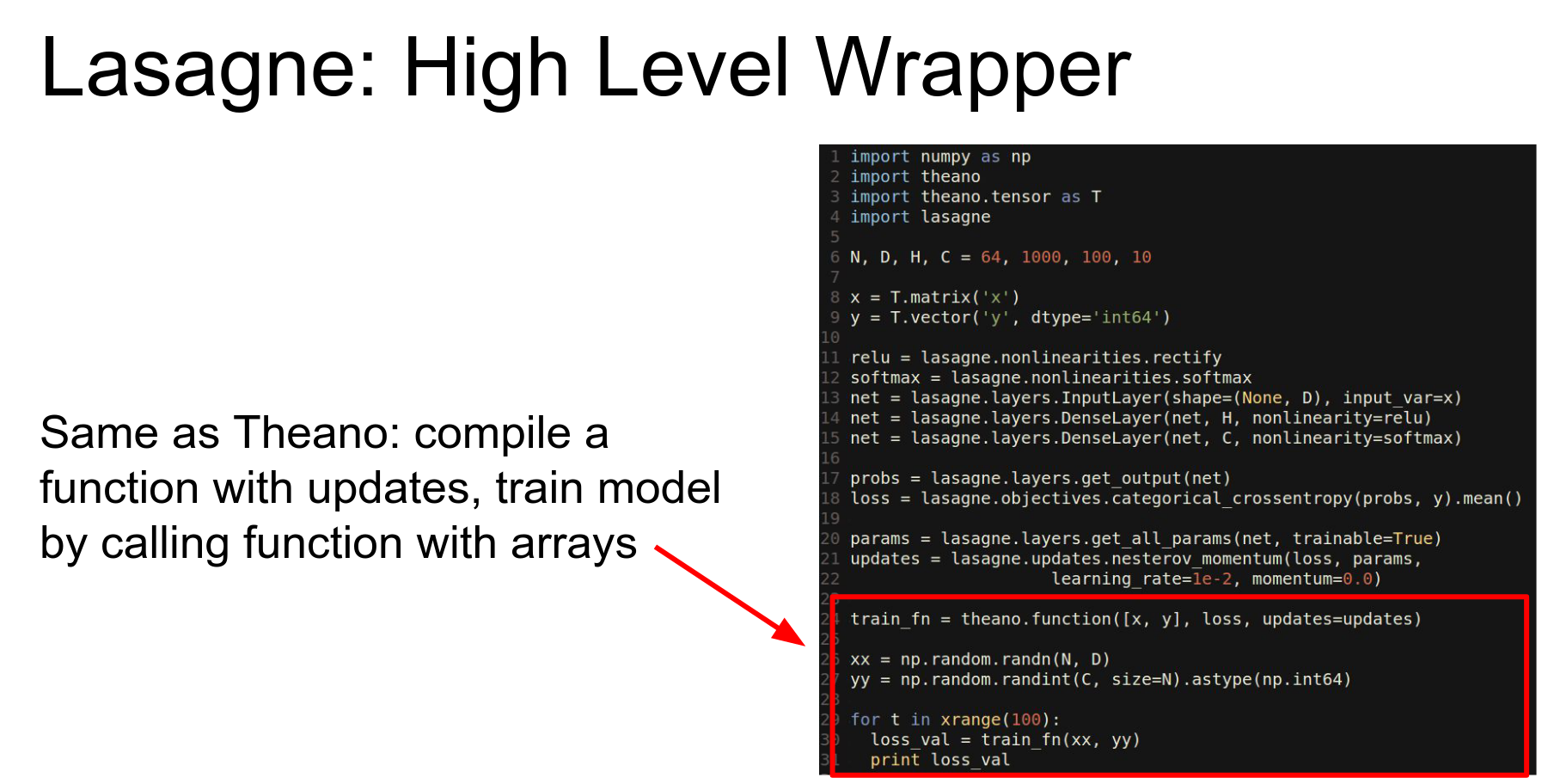
We just end up with one of these compiled Theano functions and we use it the same way as before.

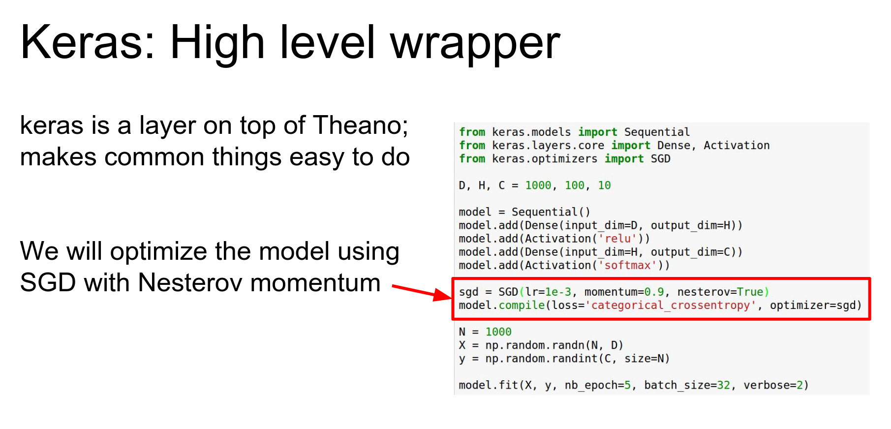
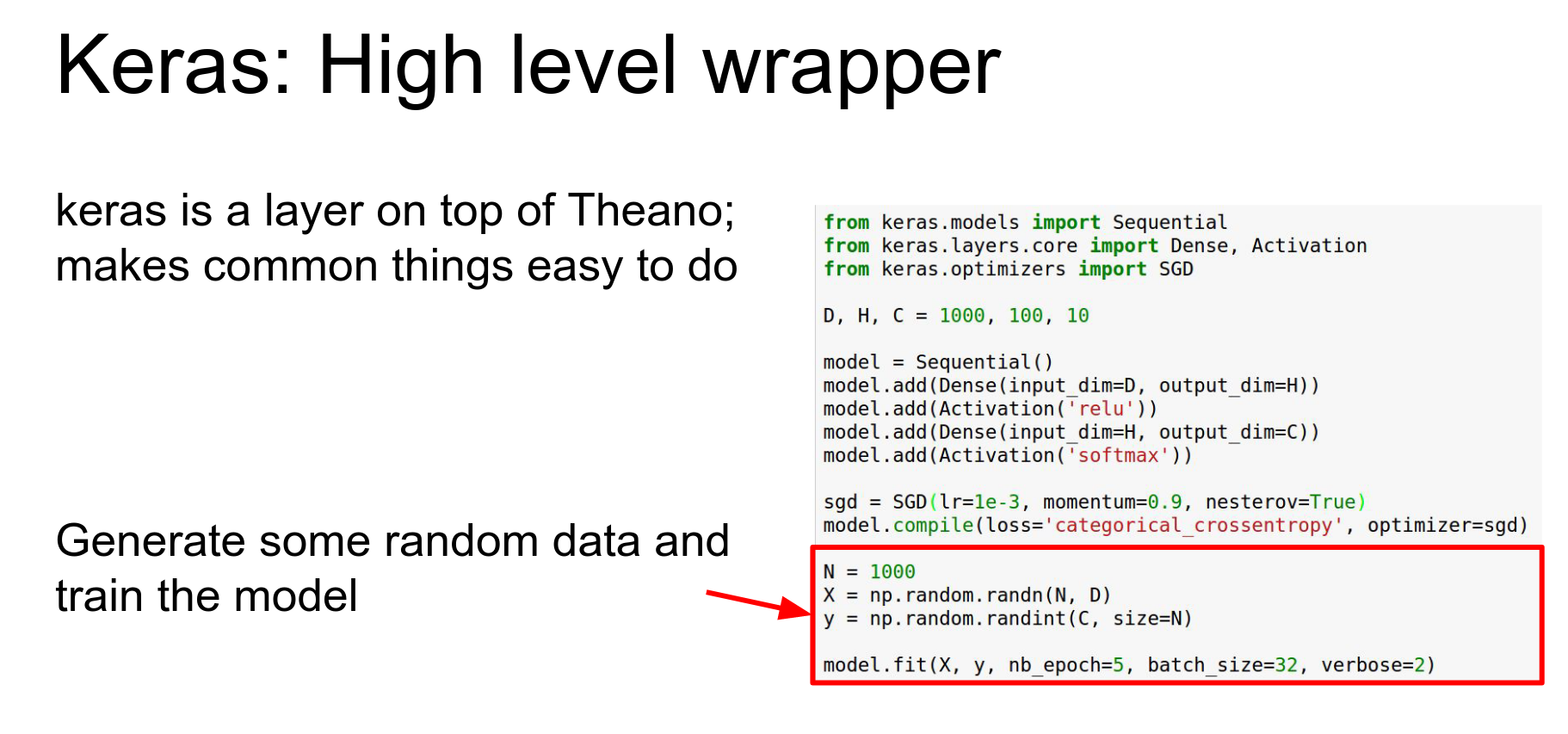
Keras: Even higher-level wrapper. Can use Theano or TensorFlow backend.

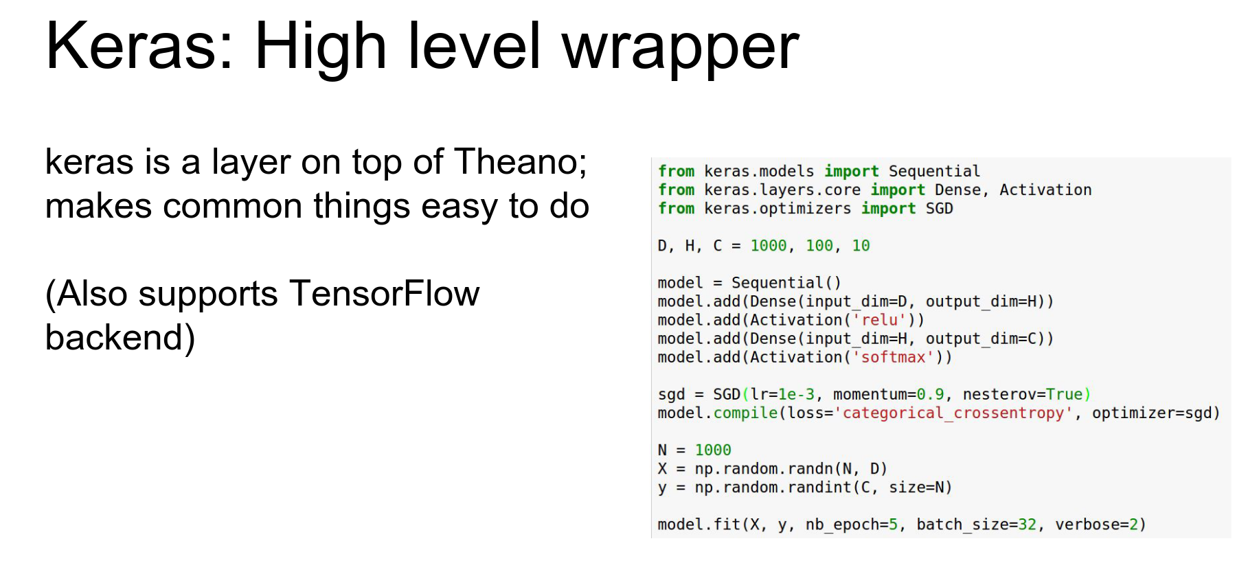
So here we're having making a sequential container and we're adding a stack of layers to it so this is kind of like torch.

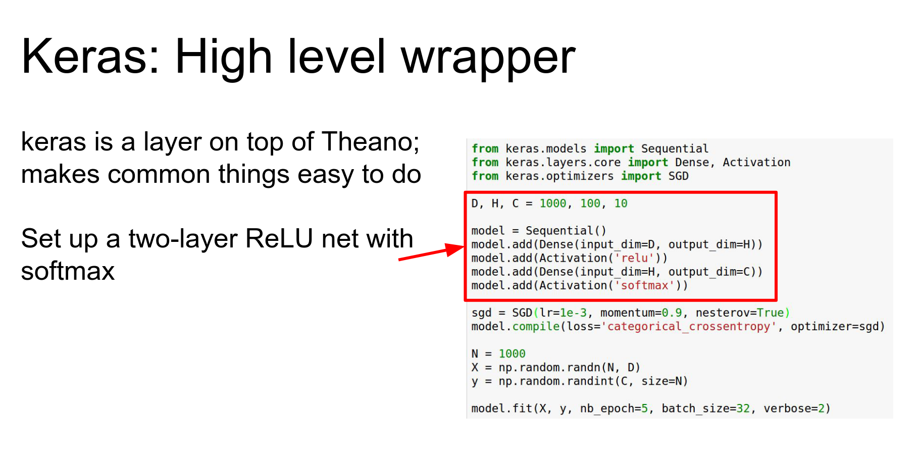
And we're having this making this SGD object that is going to actually do updates for us.

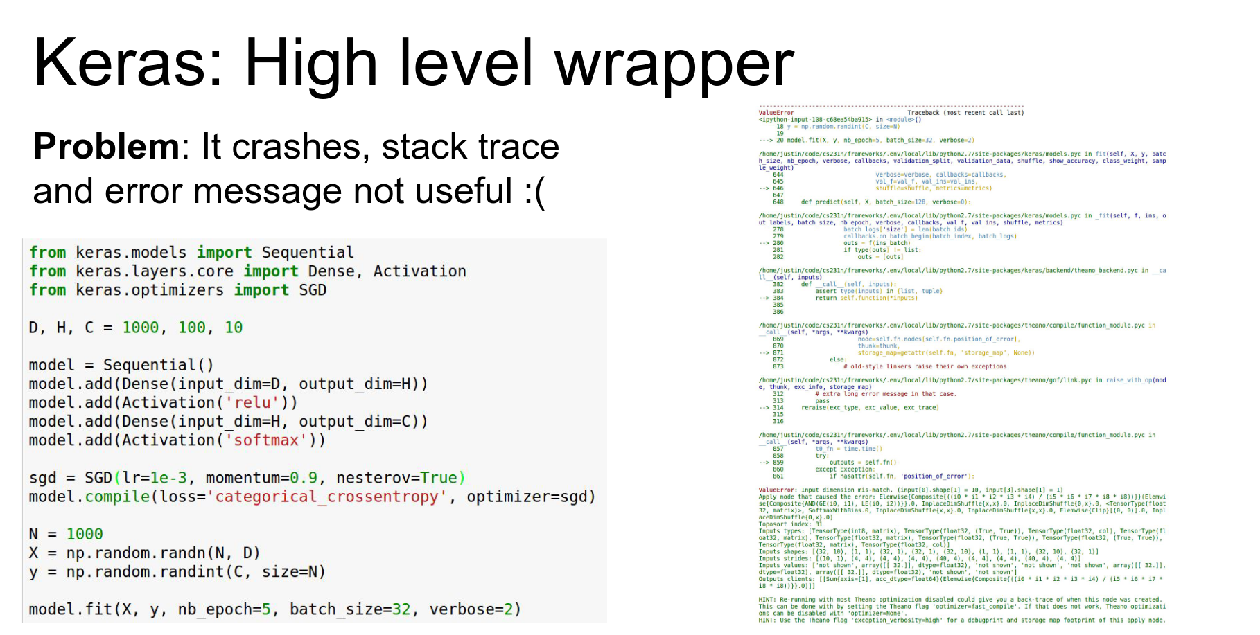
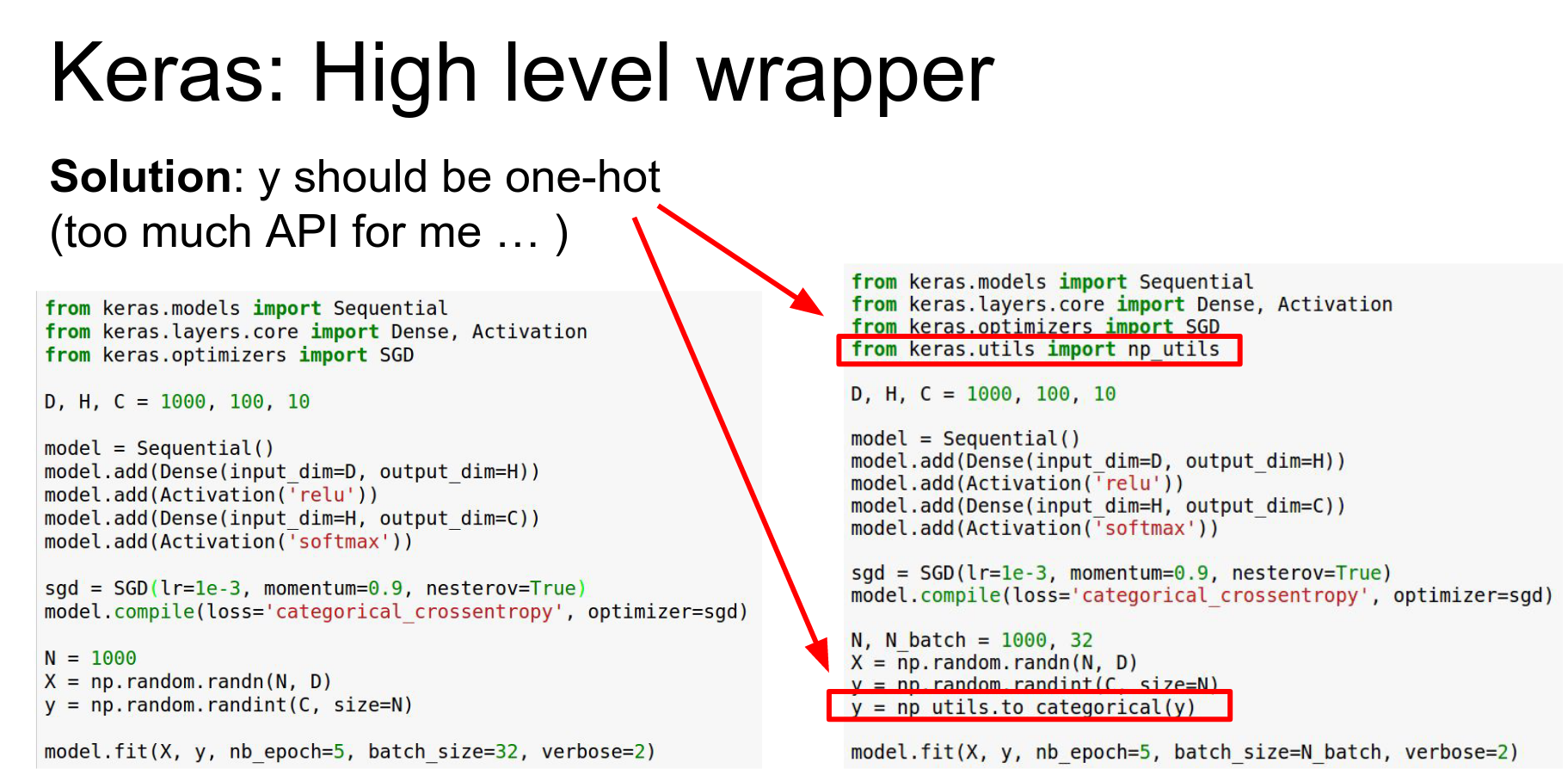
Problem: Debugging can be hard. Error messages are often cryptic stack traces from the backend.

We wrote this kind of simple looking code and Keras but because it's using Theano as a back-end it crapped out and gave us this really confusing error message.

So that's I think one of the common pain points and failure cases with anything that uses Theano as a back-end.

That debugging can be kind of hard.

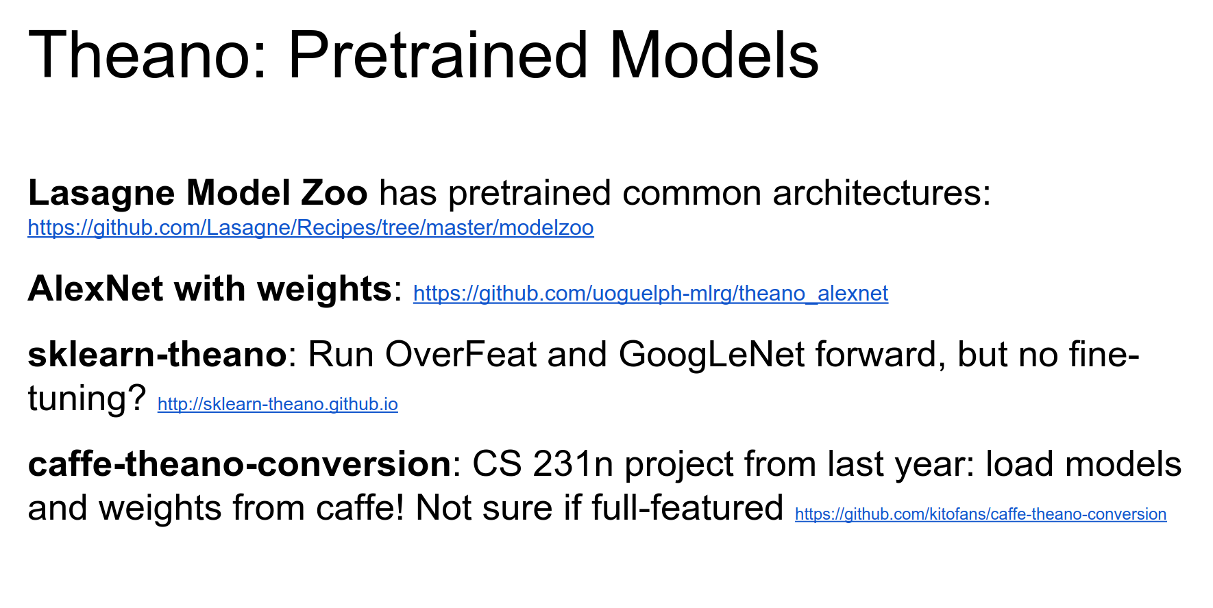
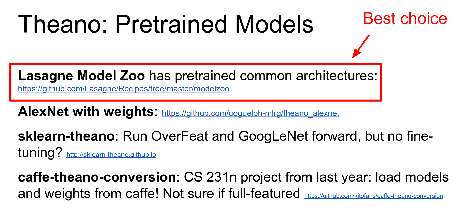
Pre-trained Models: Lasagne has a good Model Zoo (AlexNet, VGG, GoogLeNet).

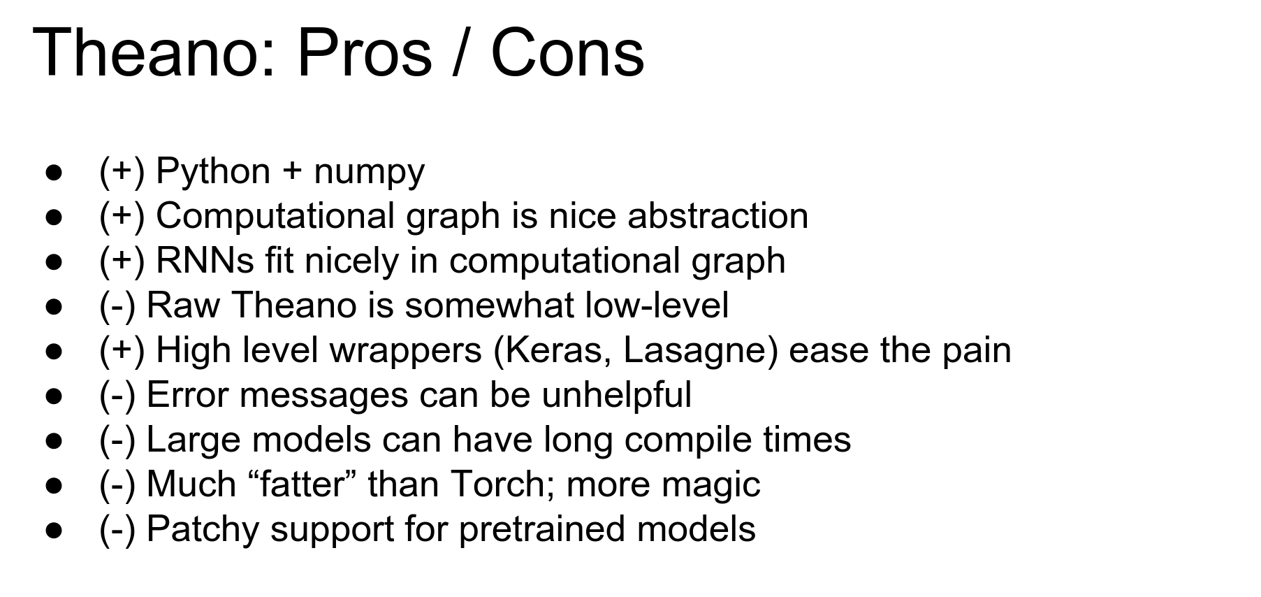
Theano Pros and Cons:

• Pros: Python/Numpy, powerful computational graphs (symbolic gradients), good for RNNs.

• Cons: Raw Theano is ugly, error messages are painful, compile times can be long for big models.

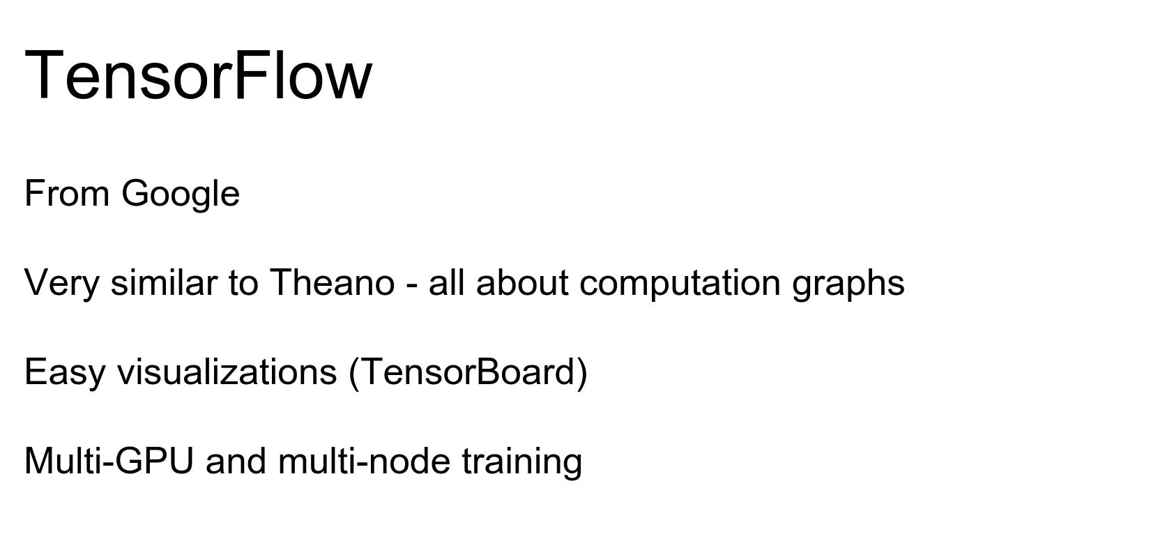
TensorFlow

TensorFlow is from Google. It is shiny, new, and everyone is excited about it.

It is very similar to Theano in that it takes the idea of a computational graph and builds everything on top of it.

TensorFlow and Theano are closely linked in concept, which is why Keras can use either as a backend.

One point to make is that TensorFlow is the first of these frameworks designed from the ground up by professional engineers (rather than academic research labs).

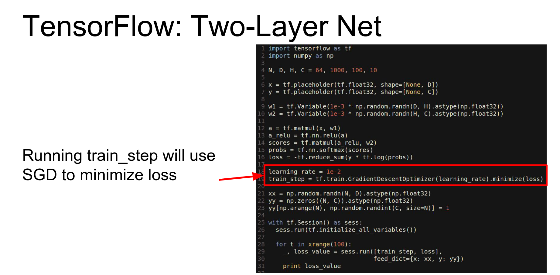
Here is our favorite two-layer ReLU network in TensorFlow.

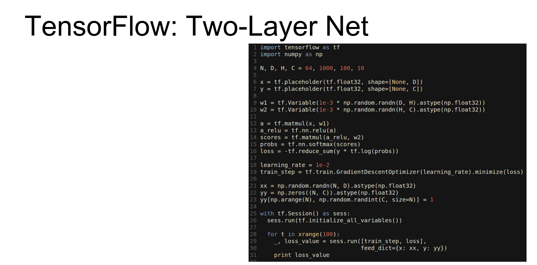
It is very similar to Theano. We import tensorflow.

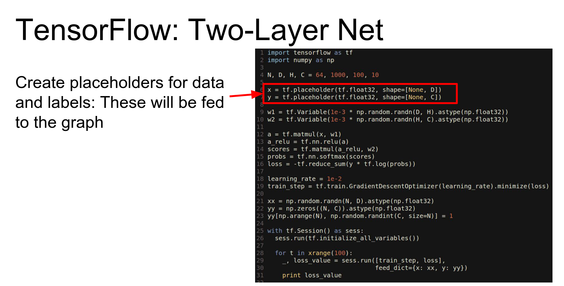
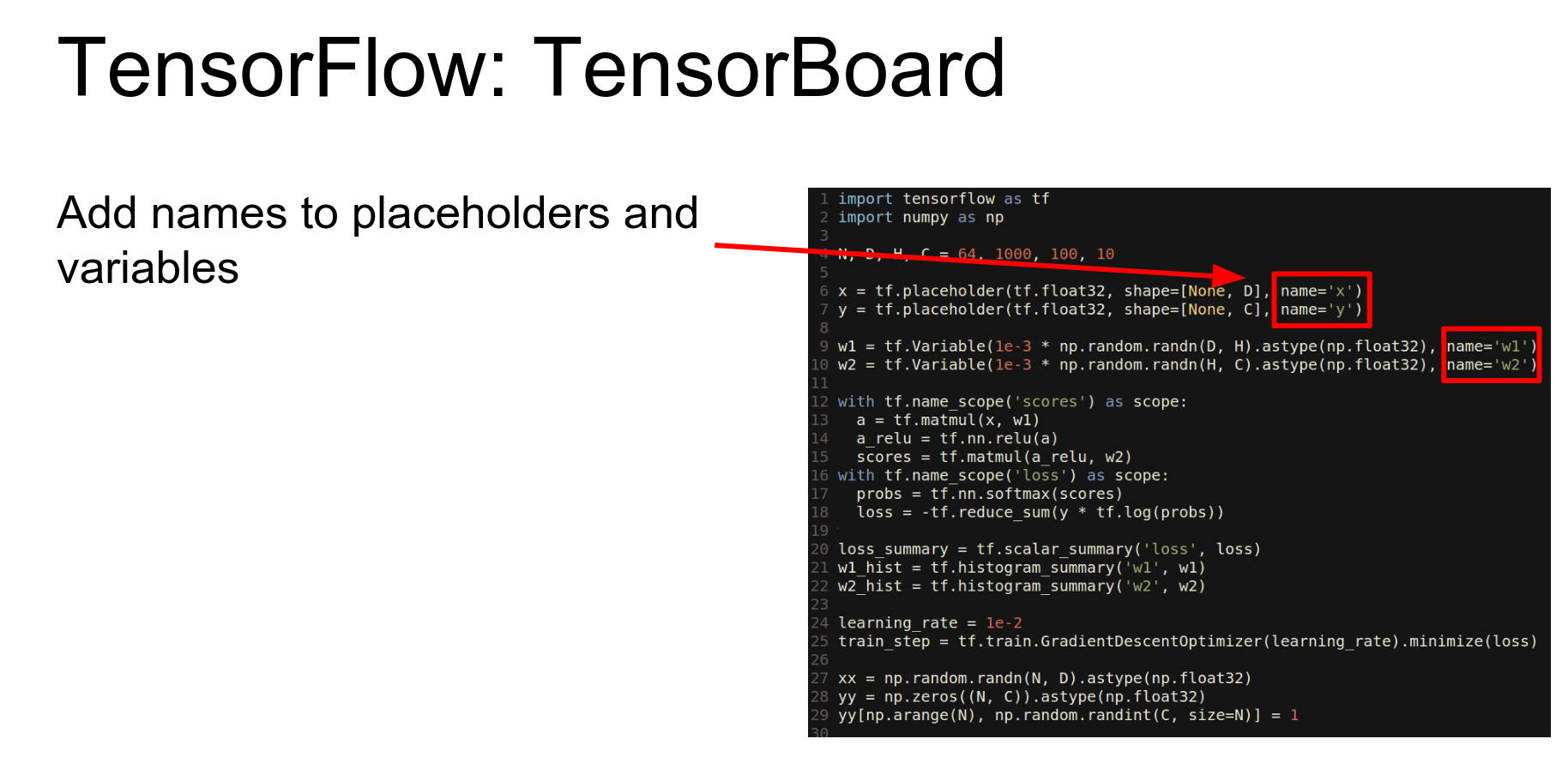
• Placeholders: Equivalent to Theano's symbolic variables (input nodes).
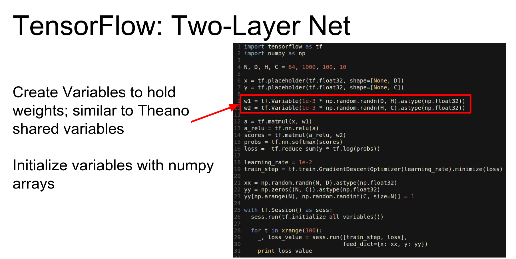
• Variables: Equivalent to Theano's shared variables (weights).

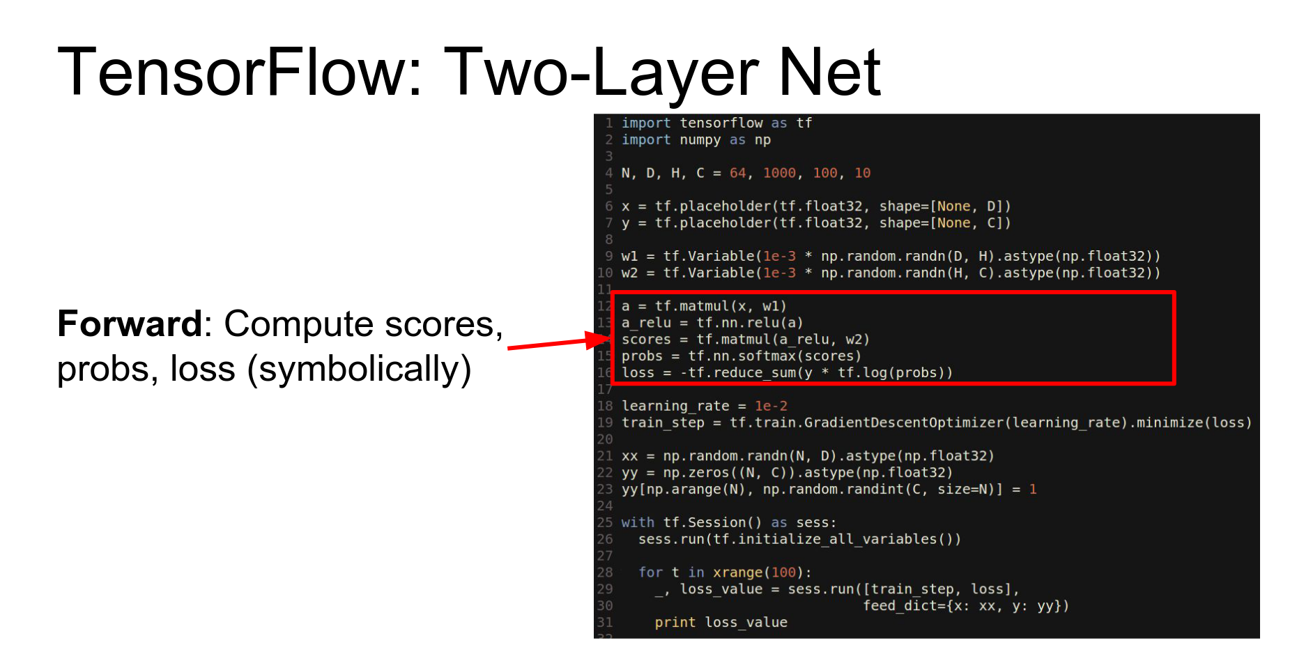
We compute the forward pass using library methods that operate symbolically to build the graph.

This part looks a bit more like Keras or Lasagne. We use a GradientDescentOptimizer and tell it to minimize the loss. We don't explicitly compute gradients or write update rules; the optimizer adds the necessary nodes to the graph.

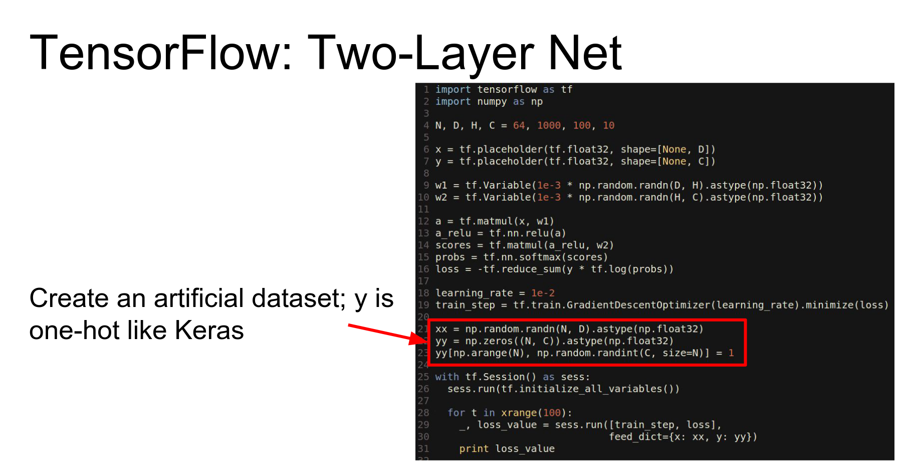
We instantiate numpy arrays for data.

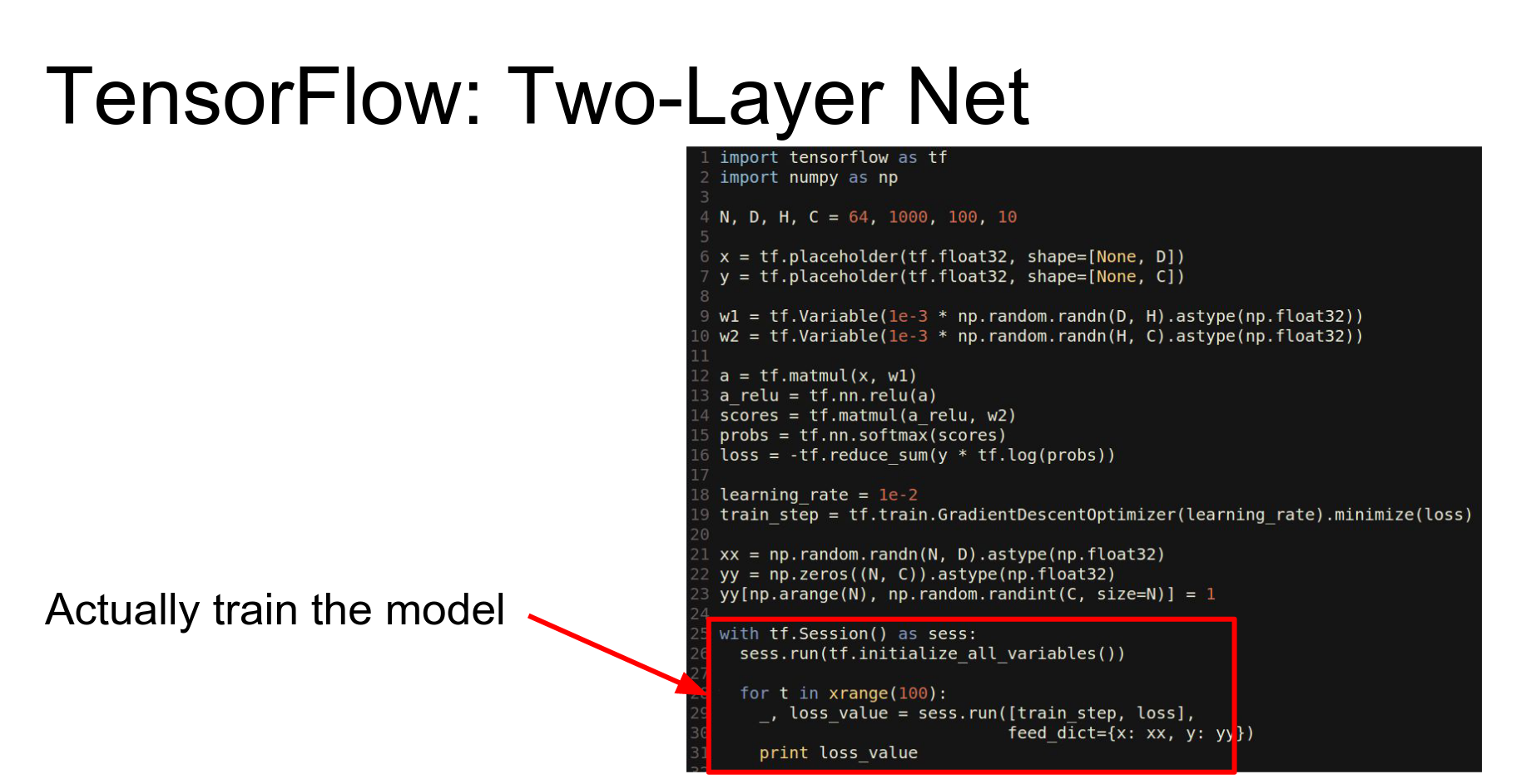
Sessions: To run code, you wrap it in a Session. The session handles the optimization and execution of the graph.

To train, we call sess.run and tell it which outputs we want (train_step, loss) and feed in the data (feed_dict).

This is equivalent to calling the compiled function in Theano.

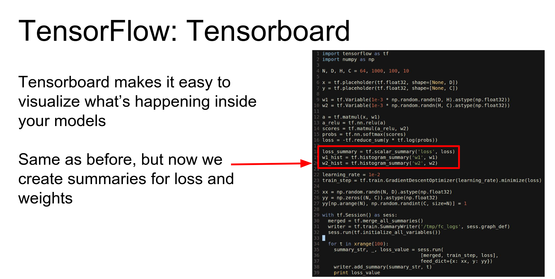
TensorBoard: One of the coolest things about TensorFlow is TensorBoard, which lets you visualize your network.

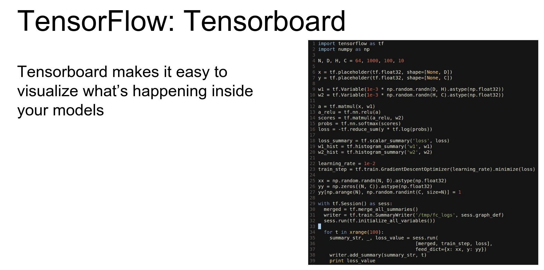
We add summary nodes to the graph: - scalar_summary for loss. - histogram_summary for weights.

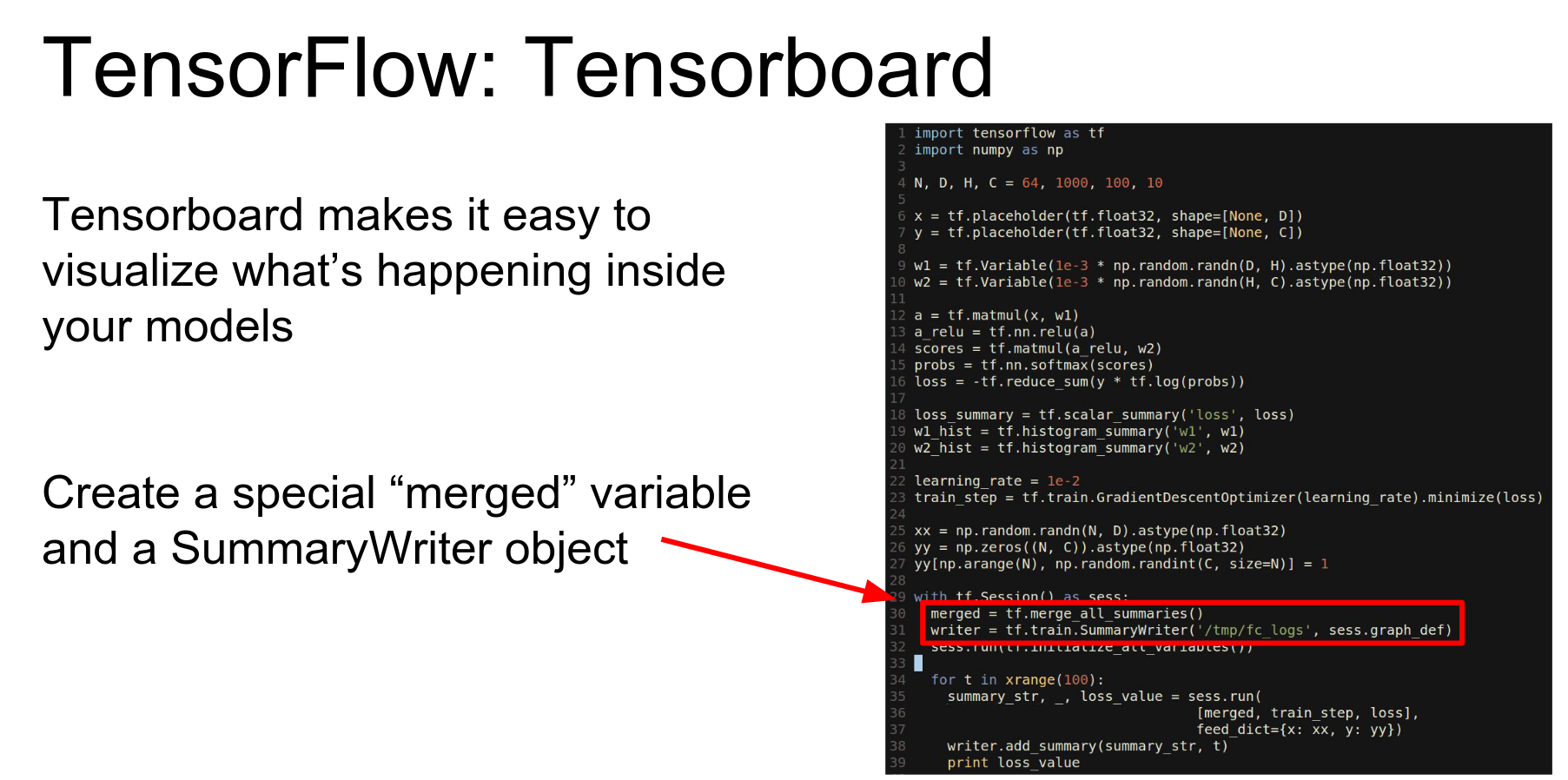
We merge all summaries and create a SummaryWriter.

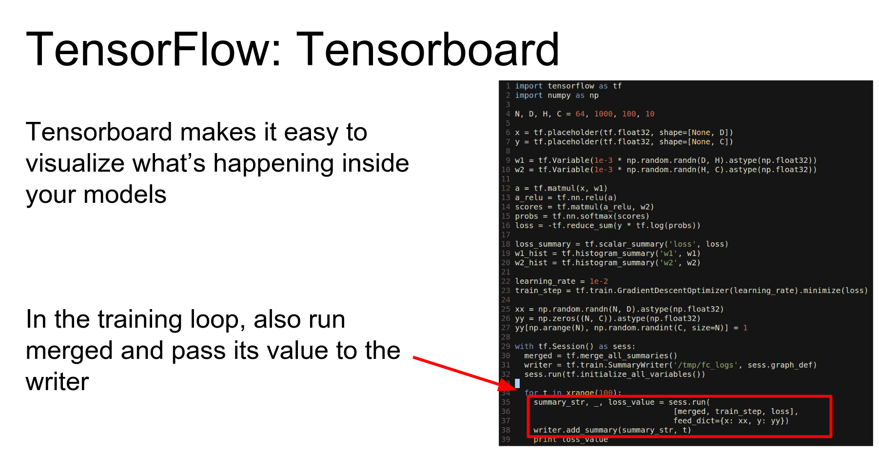
In our loop, we evaluate the merged summary object. This computes the summaries, and we write them to disk.

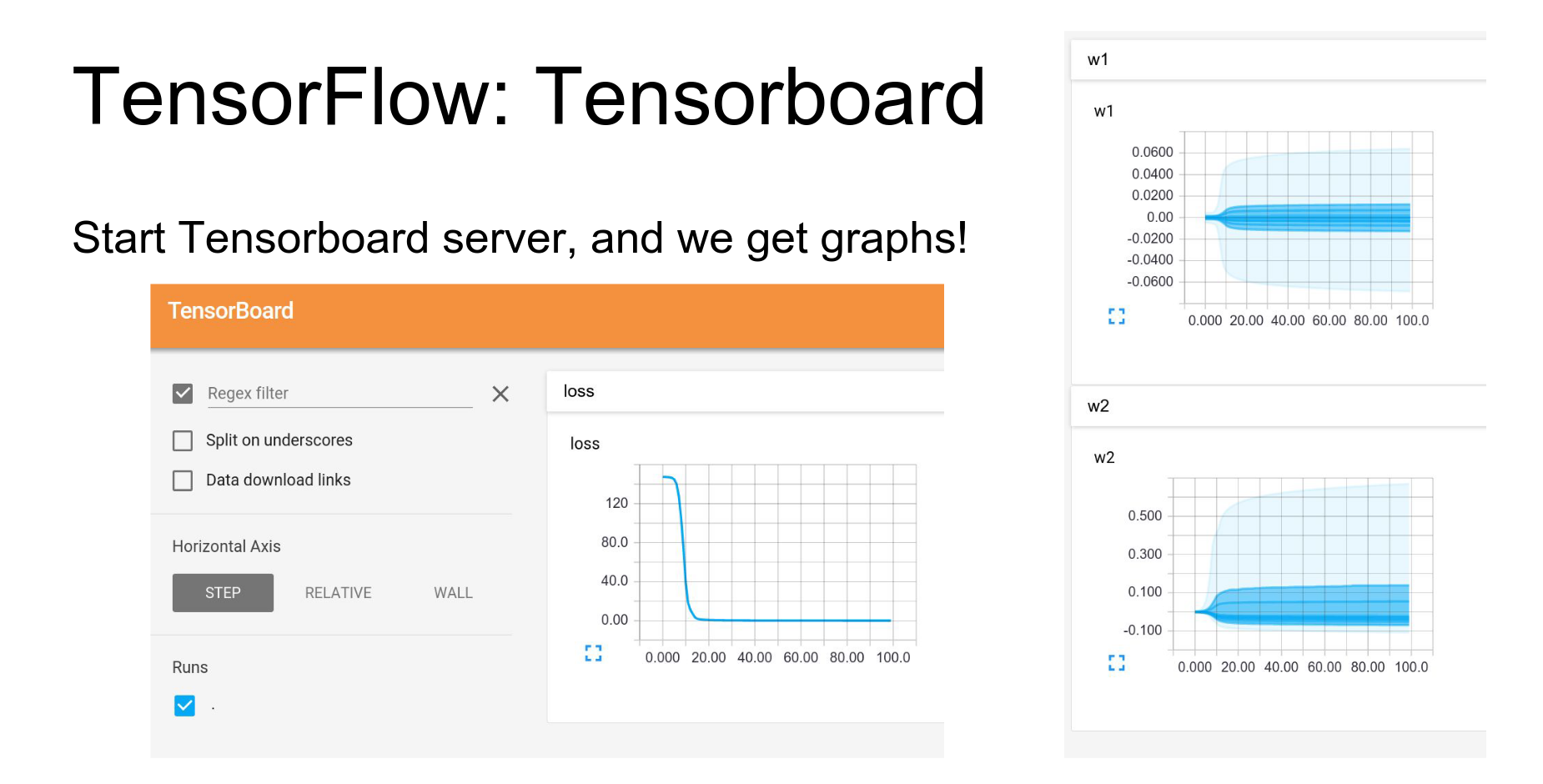
Then you start the TensorBoard web server and get beautiful visualizations.

• Loss curves.
• Histograms of weights over time.

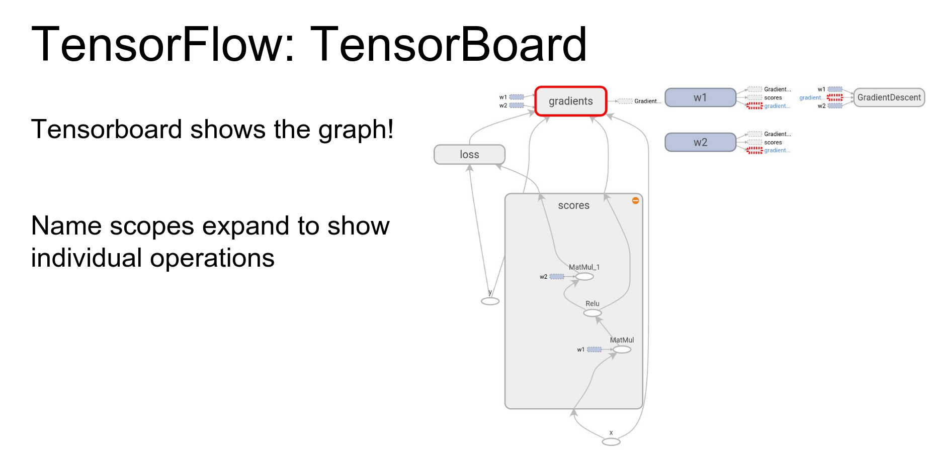
Graph Visualization: TensorBoard can also visualize your network structure.

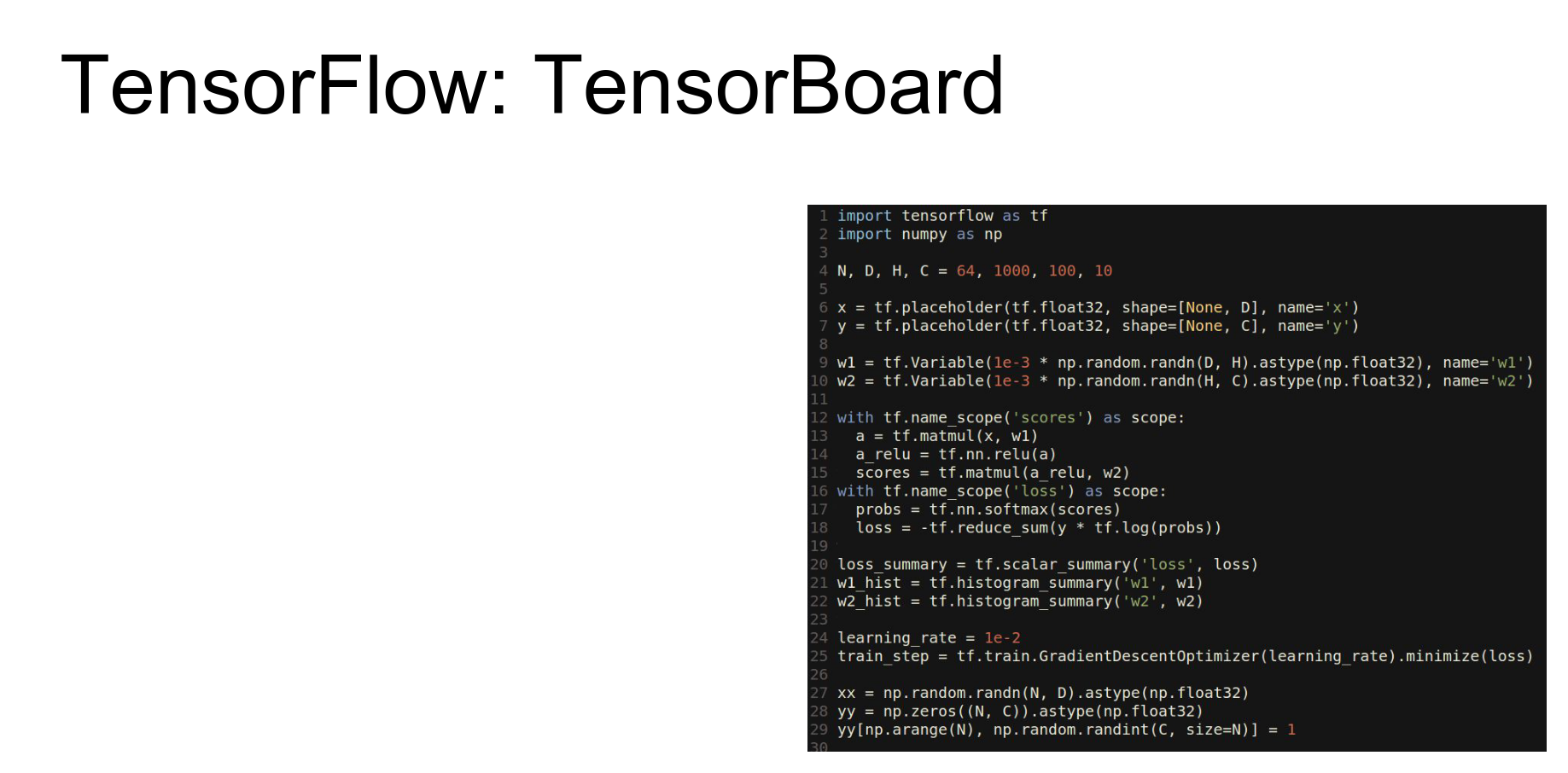
You can annotate variables with names and scope computations under namespaces to group them semantically.

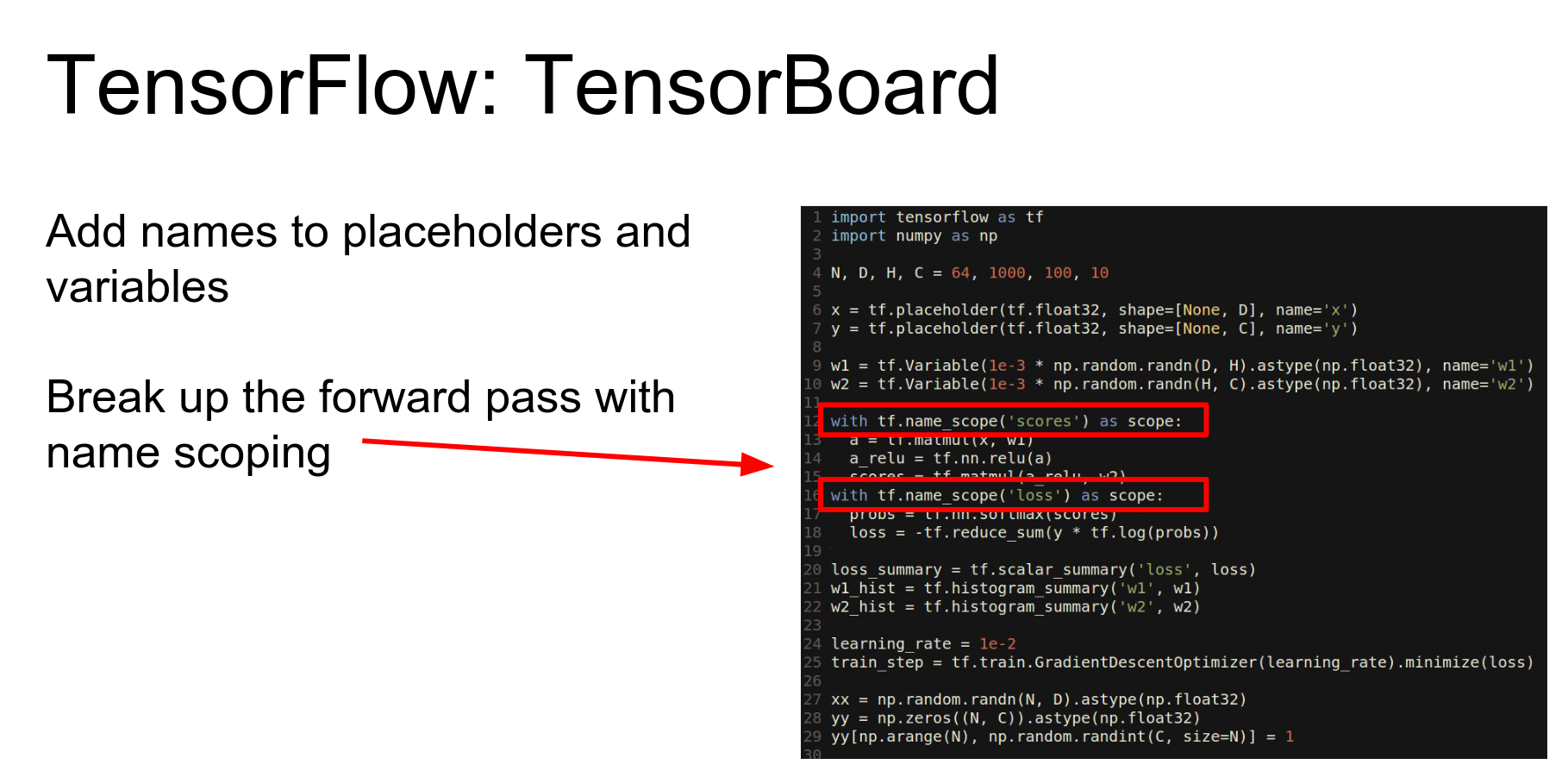
This gives you a visual representation of the computational graph, which is great for debugging.

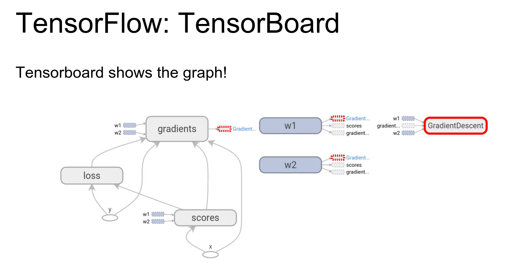
You can click into nodes to see sub-operations.

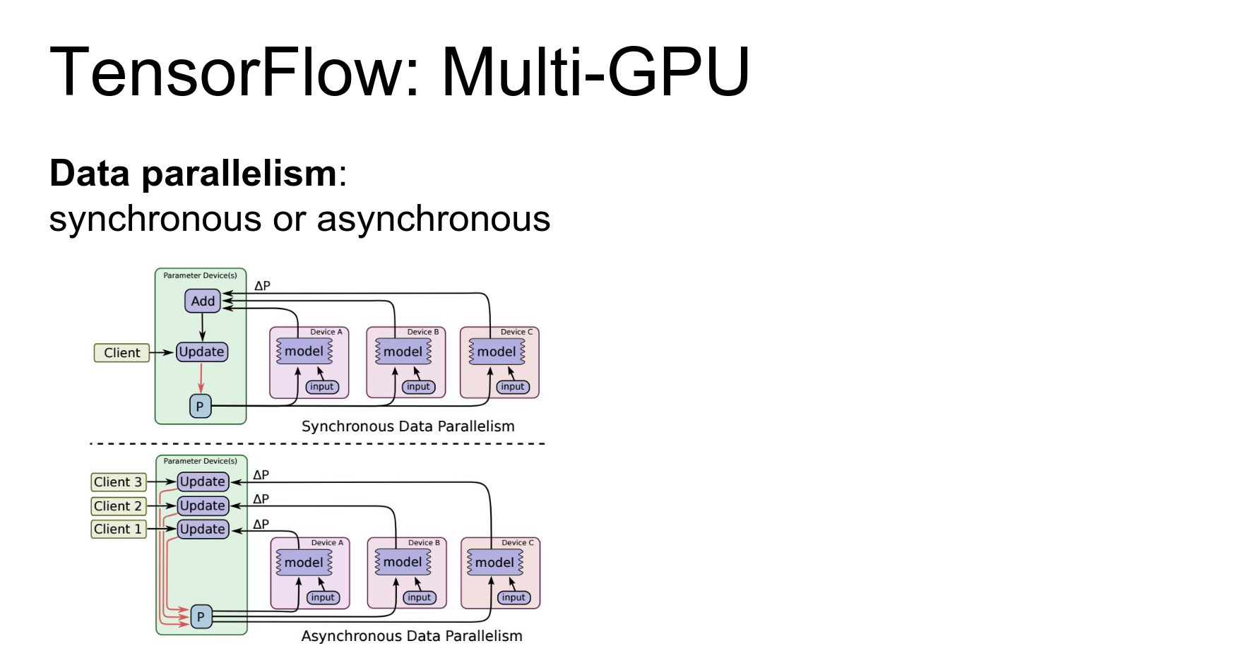
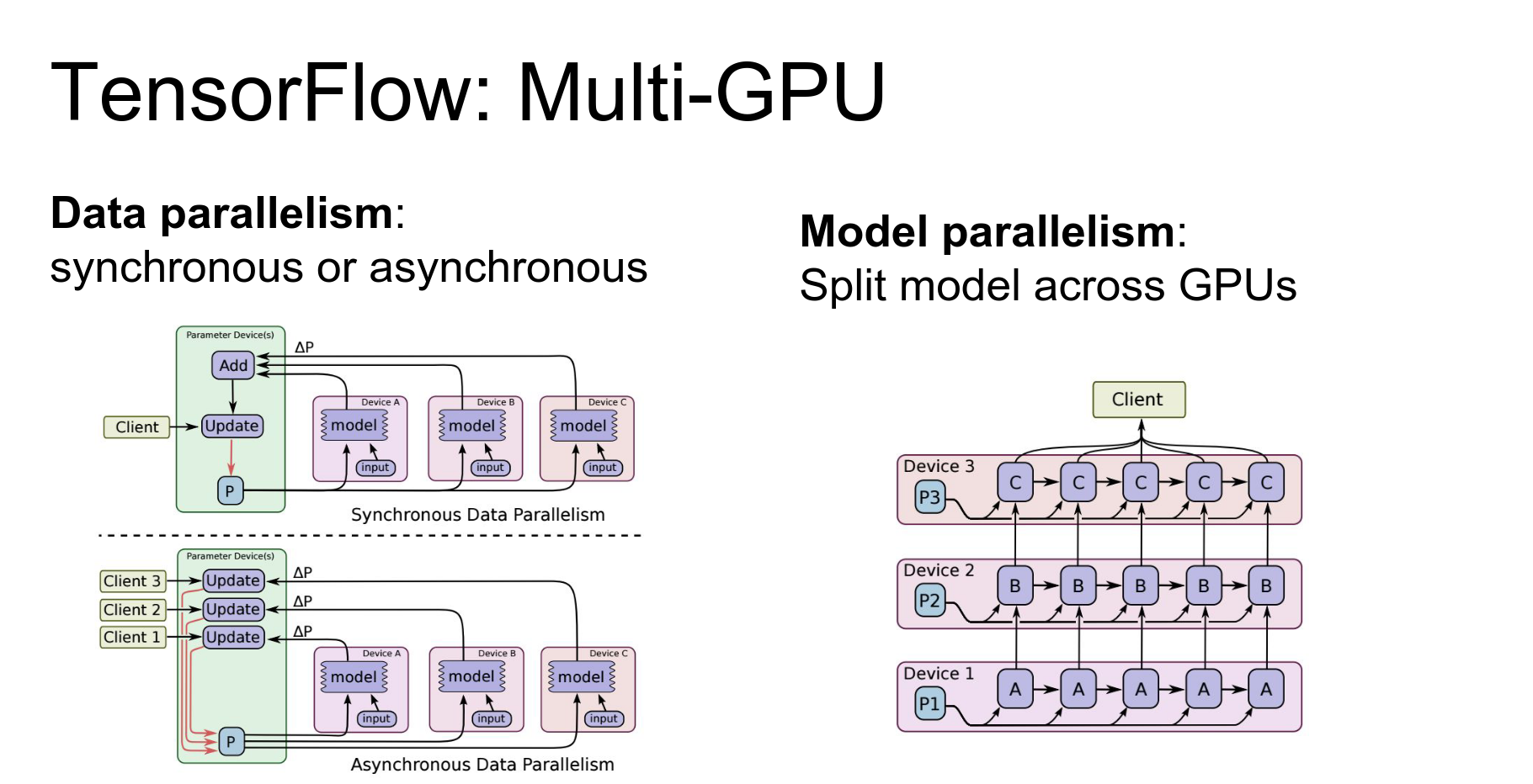
Distributed Training: TensorFlow supports data parallelism and model parallelism.

• Data Parallelism: Split mini-batch across devices.
• Model Parallelism: Split the model across devices (useful for large models or multi-layer RNNs).

You can also actually do model parallelism in TensorFlow as well that let's you split up the same model and compute different parts of the same model on different devices.

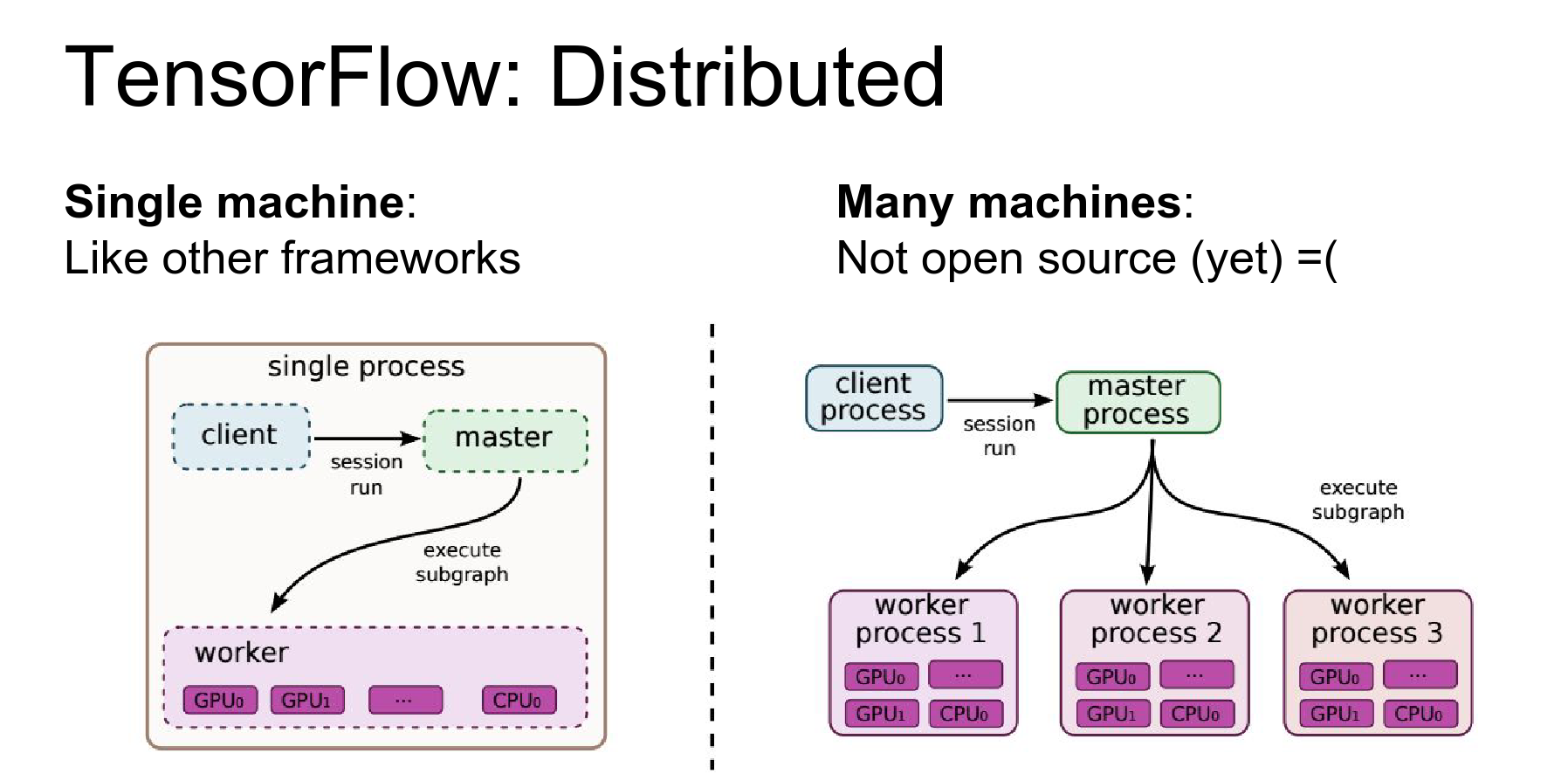
TensorFlow is the only framework that supports distributed training across multiple machines (not just multiple GPUs on one machine).

Caveat: As of today (Winter 2016), the distributed part is not open source yet. Hopefully, it will be released soon.

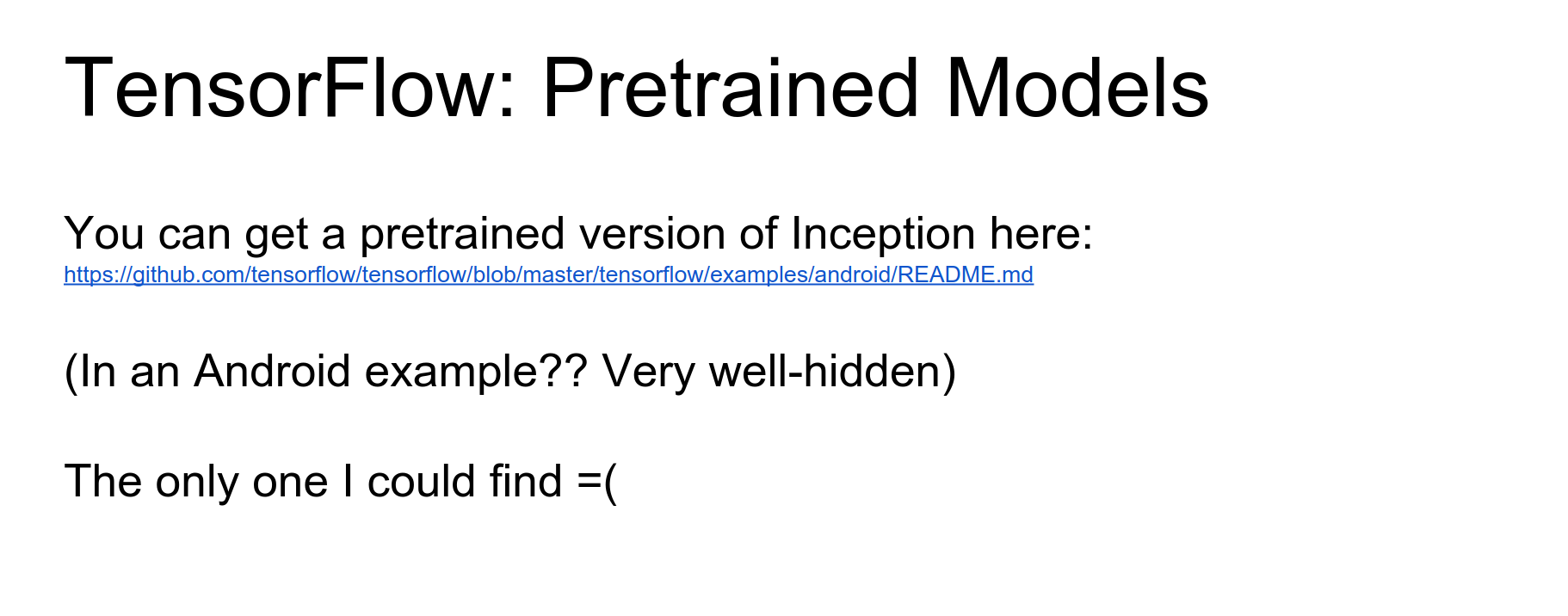
Pre-trained Models: Currently lacking. There is an Inception model in an Android demo, but not much else yet.

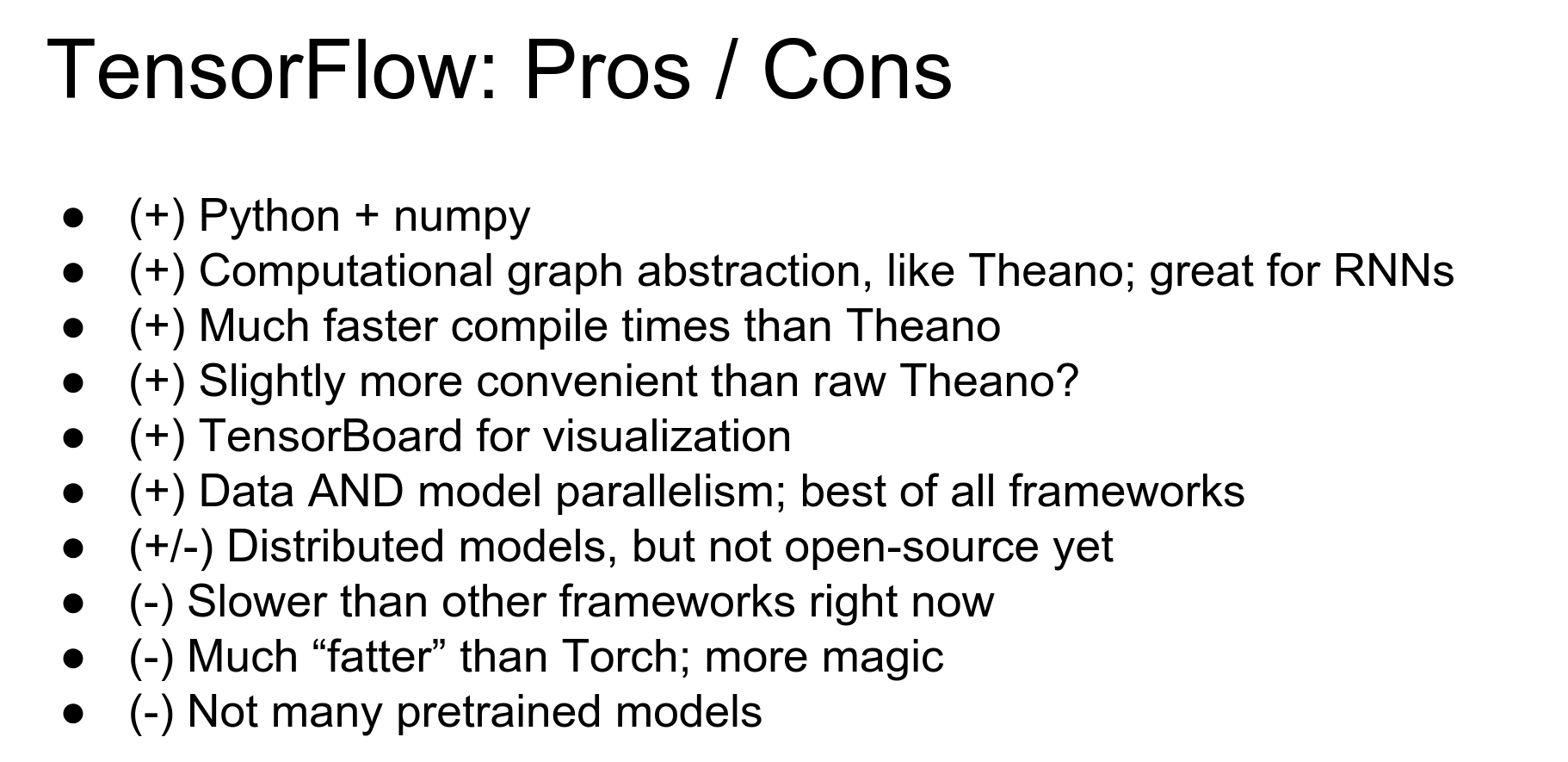
TensorFlow Pros and Cons:

• Pros: Python/Numpy, powerful computational graphs, TensorBoard is amazing, data/model parallelism.
• Cons: Slower than others (currently), distributed features not fully open source yet, lack of pre-trained models.

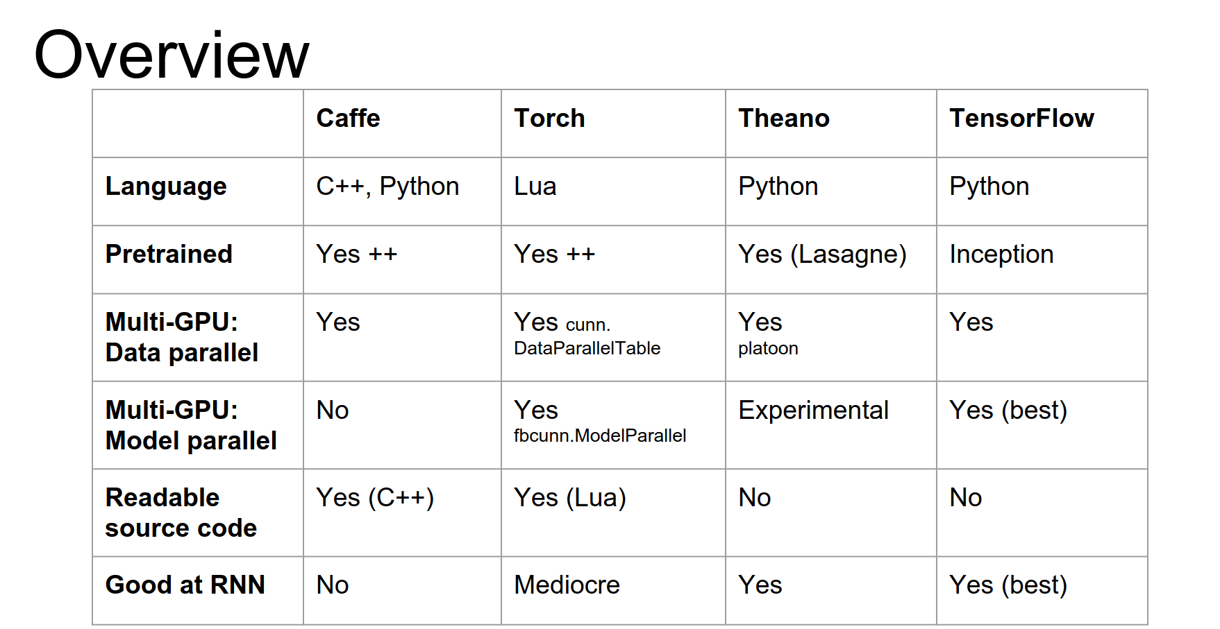
Comparison

Here is a quick overview table comparing the frameworks.

Scenarios:

1. Extract Features (AlexNet/VGG): Caffe.

1. Fine-tune AlexNet on new data: Caffe.

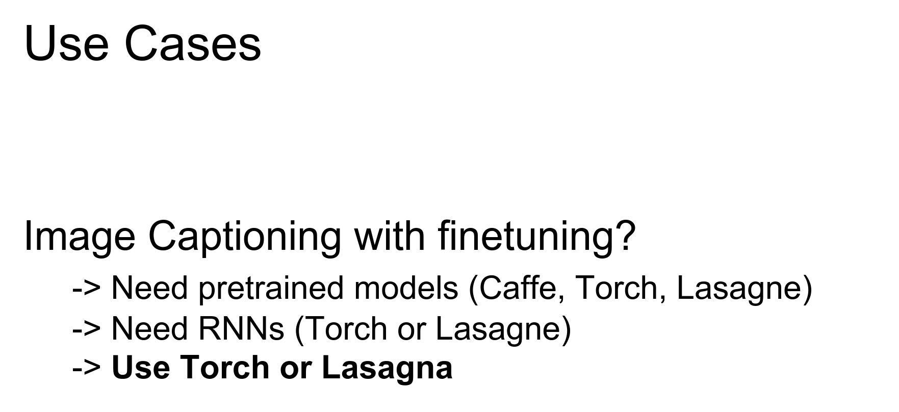
1. Image Captioning with Fine-tuning: Torch or Lasagne. (Need pre-trained models + RNNs).

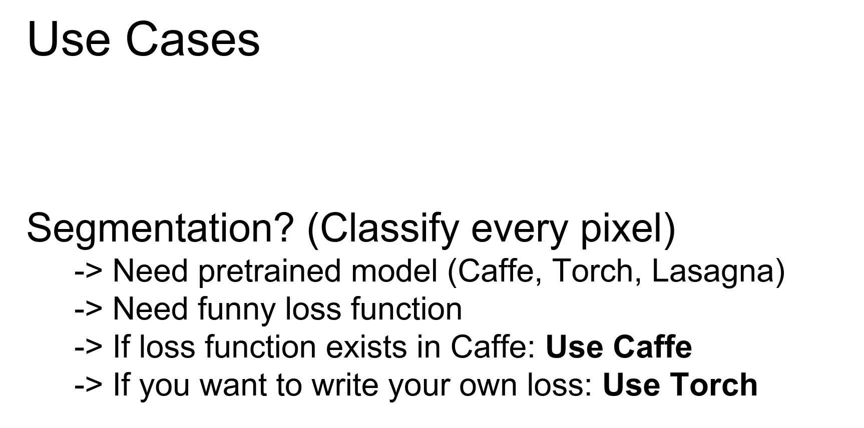
1. Semantic Segmentation: Torch. (Need pre-trained models + custom logic).

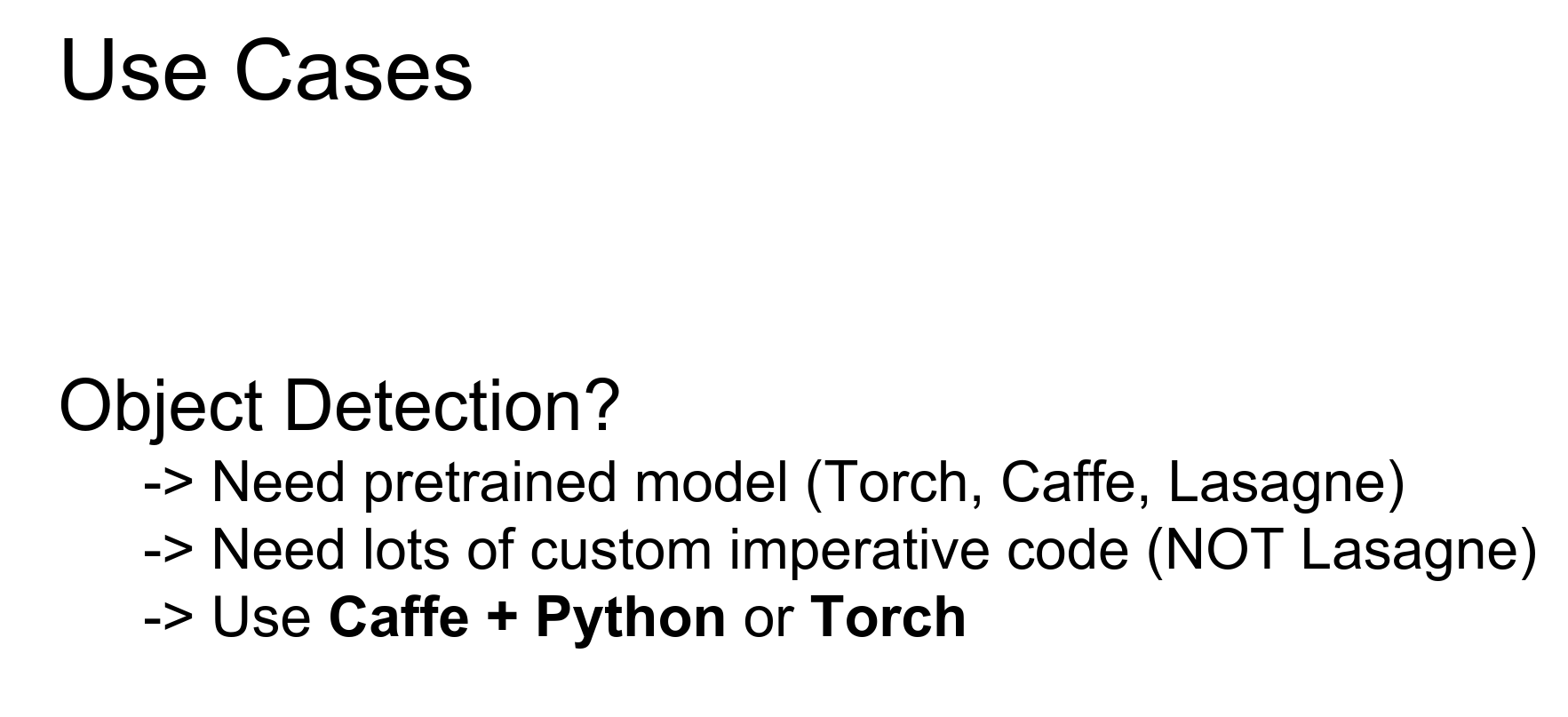
1. Object Detection: Caffe + Python, or Torch. (Complex imperative code).

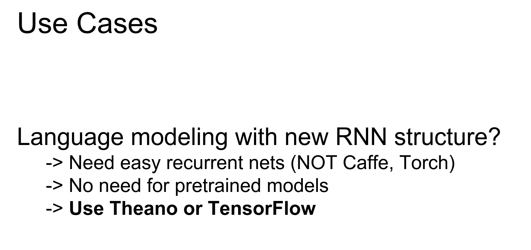
1. Language Modeling (RNNs): Theano or TensorFlow. (No pre-trained models needed, focus on recurrence).

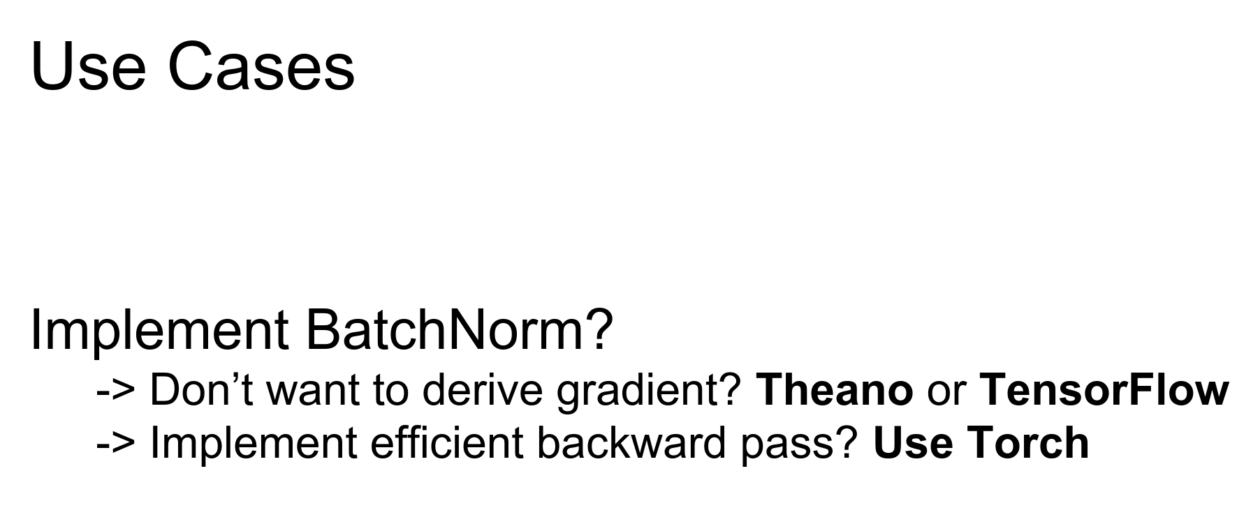
1. Implement Batch Norm (Custom Gradients): Torch. (If you want to implement efficient gradients yourself).

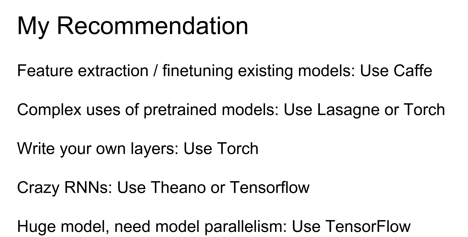
Recommendations:

• Feature Extraction / Fine-tuning: Caffe.
• Complex uses of Pre-trained Models: Lasagne or Torch.
• Writing Custom Layers: Torch.
• RNNs / Computational Graphs: Theano or TensorFlow.
• Gigantic Distributed Models: TensorFlow.

Speed: Currently, Neon (Nervana Systems) is fastest (custom assembler). Among the others using cuDNN, speed is roughly the same. TensorFlow is currently a bit slower but should improve.

Graphing: Torch has iTorch notebooks.

Down below are the extras, no time left in the lecture to cover them.

Done with lecture 12. 🍒

---

Extra: How to calculate gradients ? 🍒

In the context of deep learning and neural network training, "parsing out the AST (Abstract Syntax Tree) for calculating gradients" refers to the process of automatically differentiating the computational graph of a neural network to compute the gradients of the model parameters with respect to the loss function.Here's a more detailed explanation:

1. Computational Graph: When building a neural network in a deep learning framework like PyTorch or TensorFlow, the network is represented as a computational graph. This graph consists of nodes (representing operations like matrix multiplication, activation functions, etc.) and edges (representing the flow of tensors between operations).

2. Automatic Differentiation: To train a neural network using gradient-based optimization methods (like stochastic gradient descent), we need to compute the gradients of the model parameters with respect to the loss function. This process is known as automatic differentiation or backpropagation.

3. Abstract Syntax Tree (AST): The computational graph of a neural network can be represented as an AST, which is a tree-like data structure that captures the structure of the computations performed by the network. Each node in the AST represents an operation, and the edges represent the dependencies between the operations.

4. Parsing the AST: To compute the gradients, the deep learning framework needs to "parse" the AST of the computational graph. This involves traversing the AST, identifying the operations, and applying the chain rule of differentiation to compute the gradients of the model parameters with respect to the loss function.

5. Gradient Calculation: By parsing the AST, the deep learning framework can automatically compute the gradients of the model parameters with respect to the loss function. This is done by applying the chain rule of differentiation, starting from the output of the network and working backwards through the computational graph.

The ability to automatically differentiate the computational graph and compute the gradients is a key feature of modern deep learning frameworks like PyTorch and TensorFlow. It allows developers to focus on defining the neural network architecture and the loss function, without having to manually derive and implement the gradient calculations.This automatic differentiation process, enabled by parsing the AST of the computational graph, is a crucial component that allows deep learning models to be trained efficiently using gradient-based optimization methods.

---