13. Segmentation

Part of CS231n Winter 2016

---

Lecture 13: Segmentation and Attention

Assignment 3 is due tonight. Arguably it was easier than assignment 2, so hopefully, that gives you more time to work on your projects.

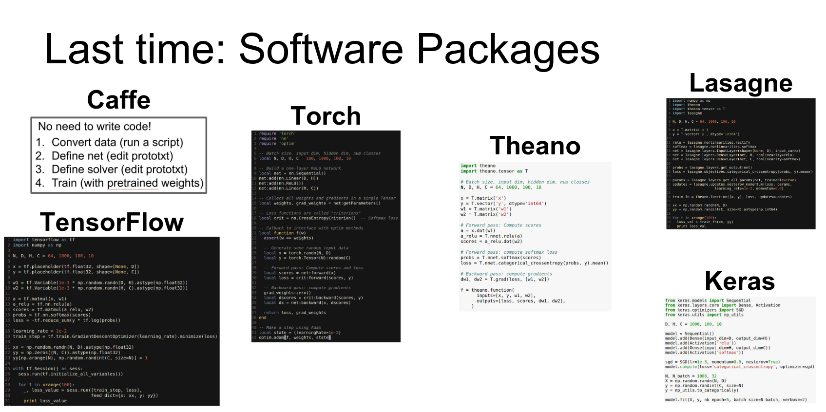
Last time we had a whirlwind tour of all the common software packages that people use for deep learning.

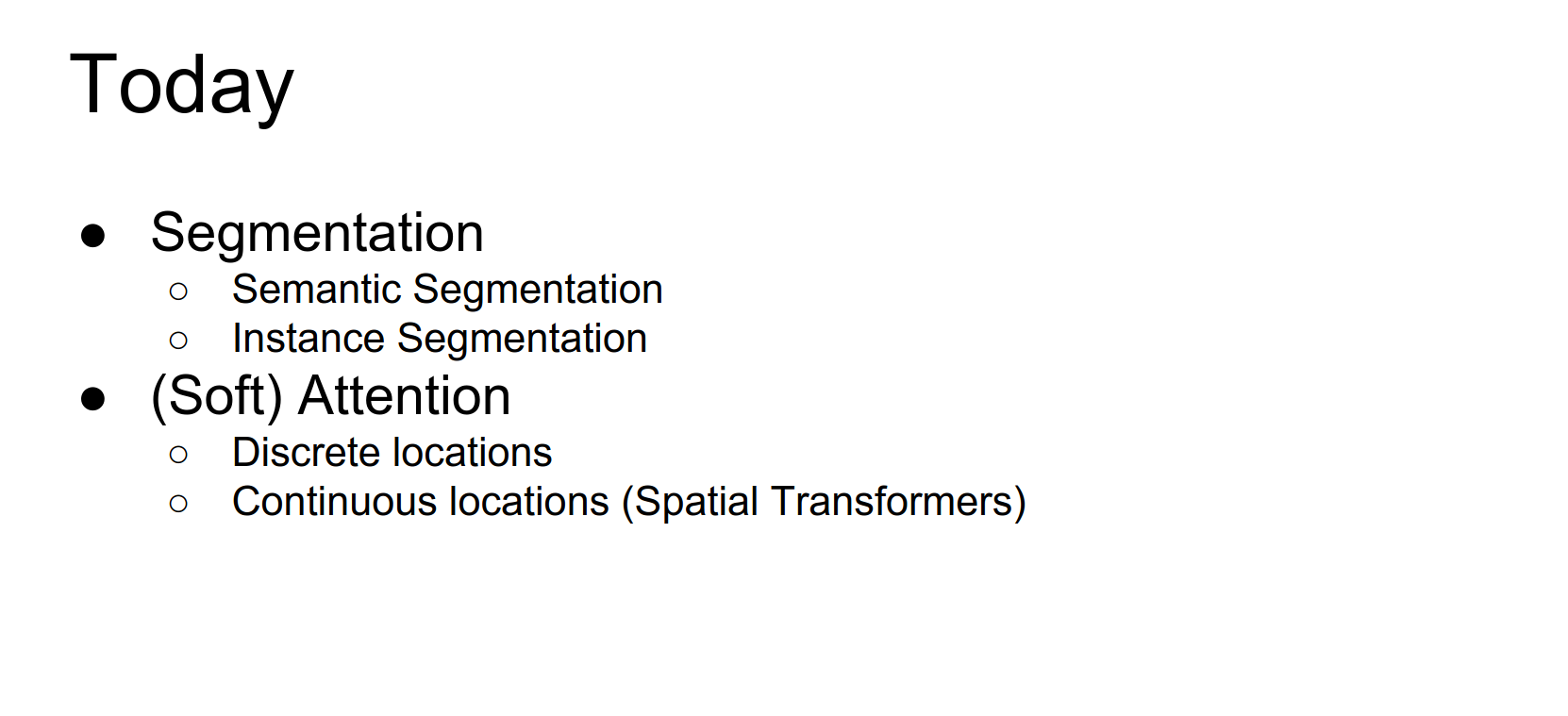
Today we're going to talk about two other topics: Segmentation and Attention.

Within segmentation, there are two sub-problems: Semantic Segmentation and Instance Segmentation. Within attention, we'll discuss Soft Attention and Hard Attention.

This is the ImageNet classification error chart. In 2012 AlexNet, 2013 ZF, 2014 GoogLeNet/VGG, and 2015 ResNet won the challenge.

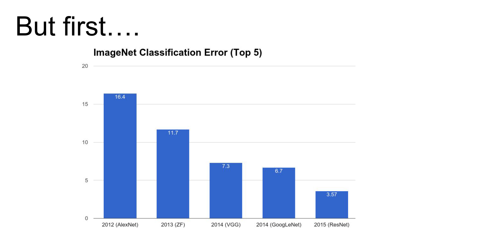
As of today, there's a new ImageNet result. Google achieved state-of-the-art on ImageNet with 3.08% top-5 error, which is crazy.

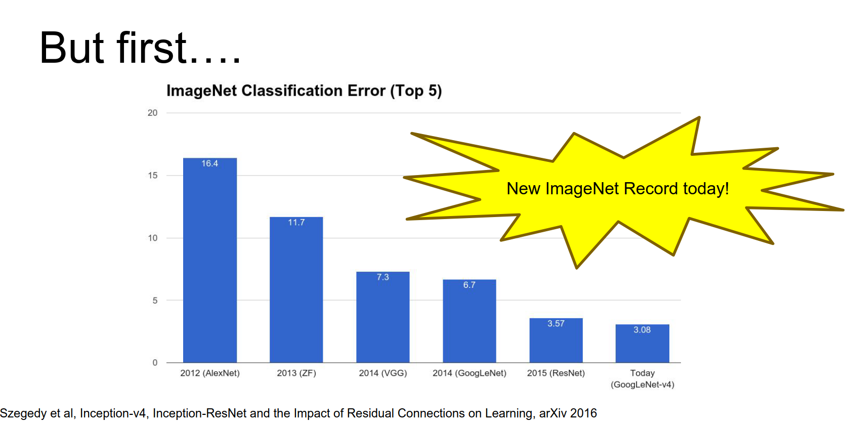
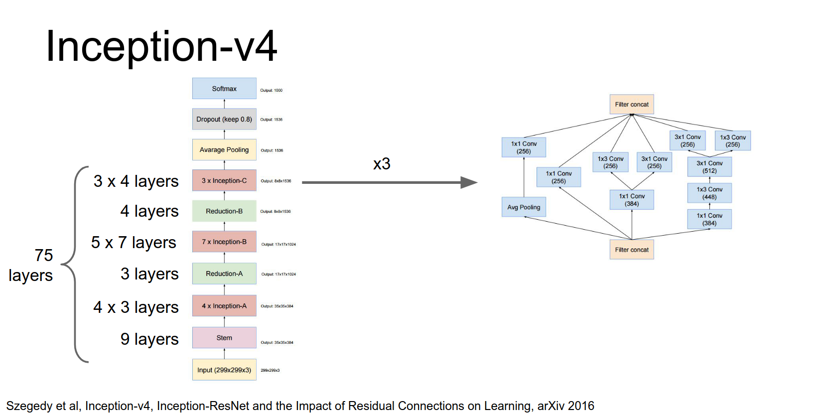
They did this with Inception-v4.

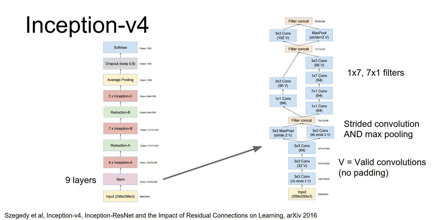
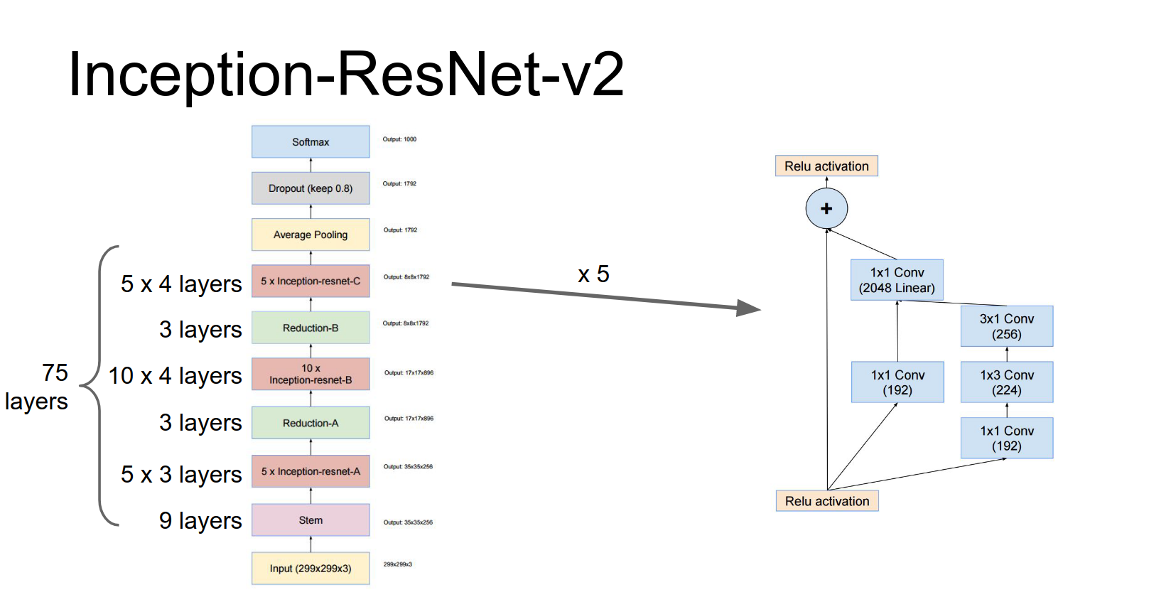
Inception-v4

This is a monster network.

It has repeated modules. A couple of interesting things:

• They use valid convolutions (no padding) in the stem.
• They perform strided convolution and max pooling in parallel to downsample, then concatenate.
• They use asymmetric filters (\(1 \times 7\) and \(7 \times 1\)) and \(1 \times 1\) bottlenecks to reduce computational cost.

They have four of these inception modules, then a downsampling module.

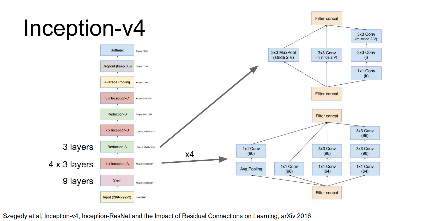
Then seven of these modules, and another downsampling module.

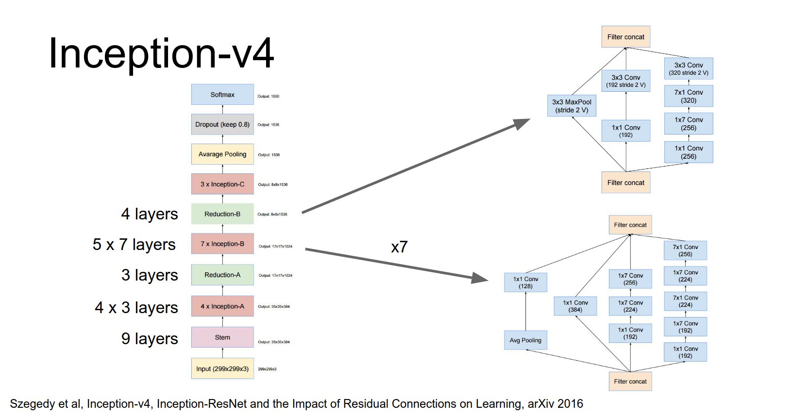
Then three more modules, and finally global average pooling and a fully connected layer.

They also proposed Inception-ResNet, which combines the Inception architecture with residual connections.

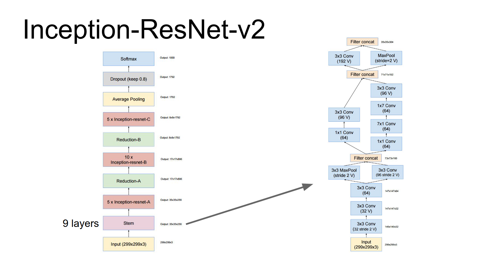These repeated inception blocks that they repeat throughout the network, they actually have these residual connections.

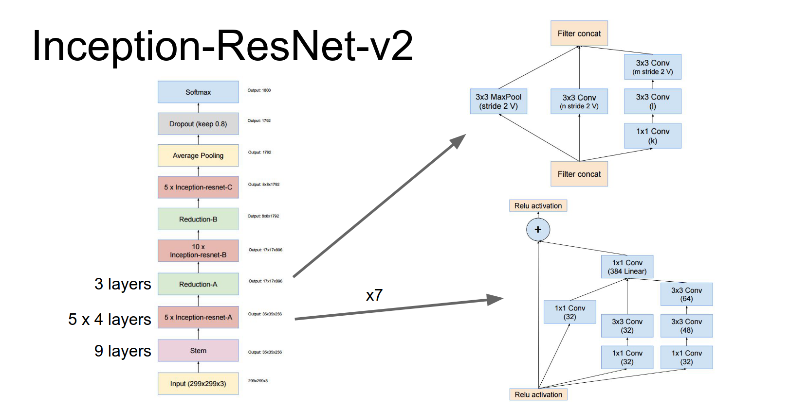
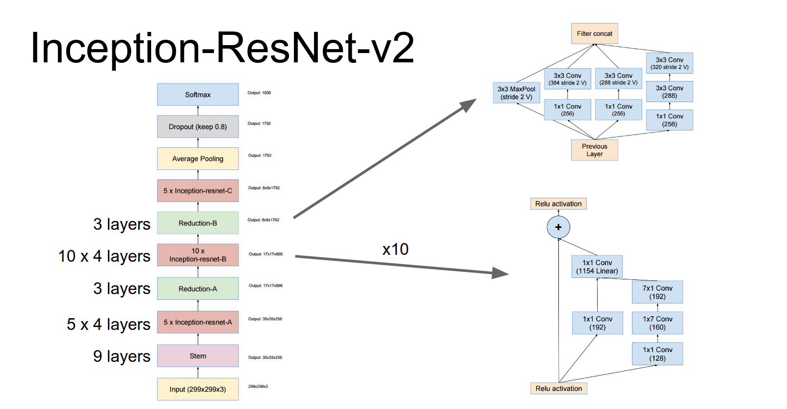
When you add it all up, it's about 75 layers deep.

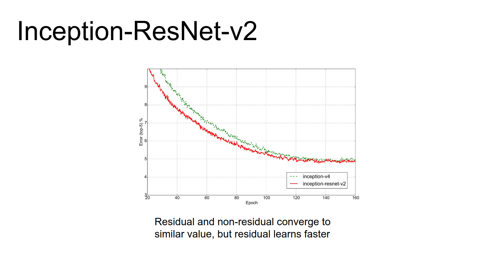
Both Inception-v4 and Inception-ResNet perform about the same, though Inception-ResNet converges faster.

The raw numbers on the x axis here these are epochs on ImageNet these things are being trained for a 160 epochs on ImageNet so that's a lot of training time.

Now, let's move on to today's topics.

Segmentation

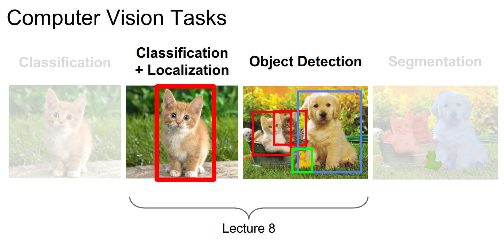
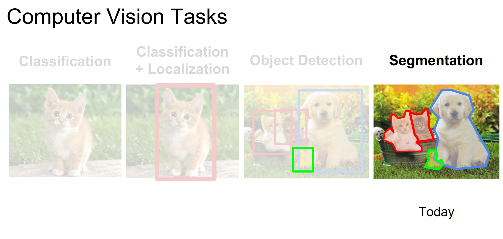
We've talked about classification, localization, and detection. Today we focus on segmentation.

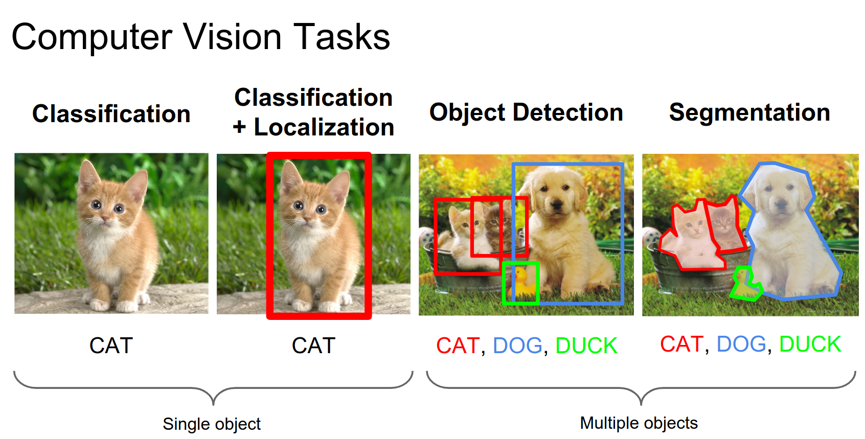
There are two main types of segmentation:

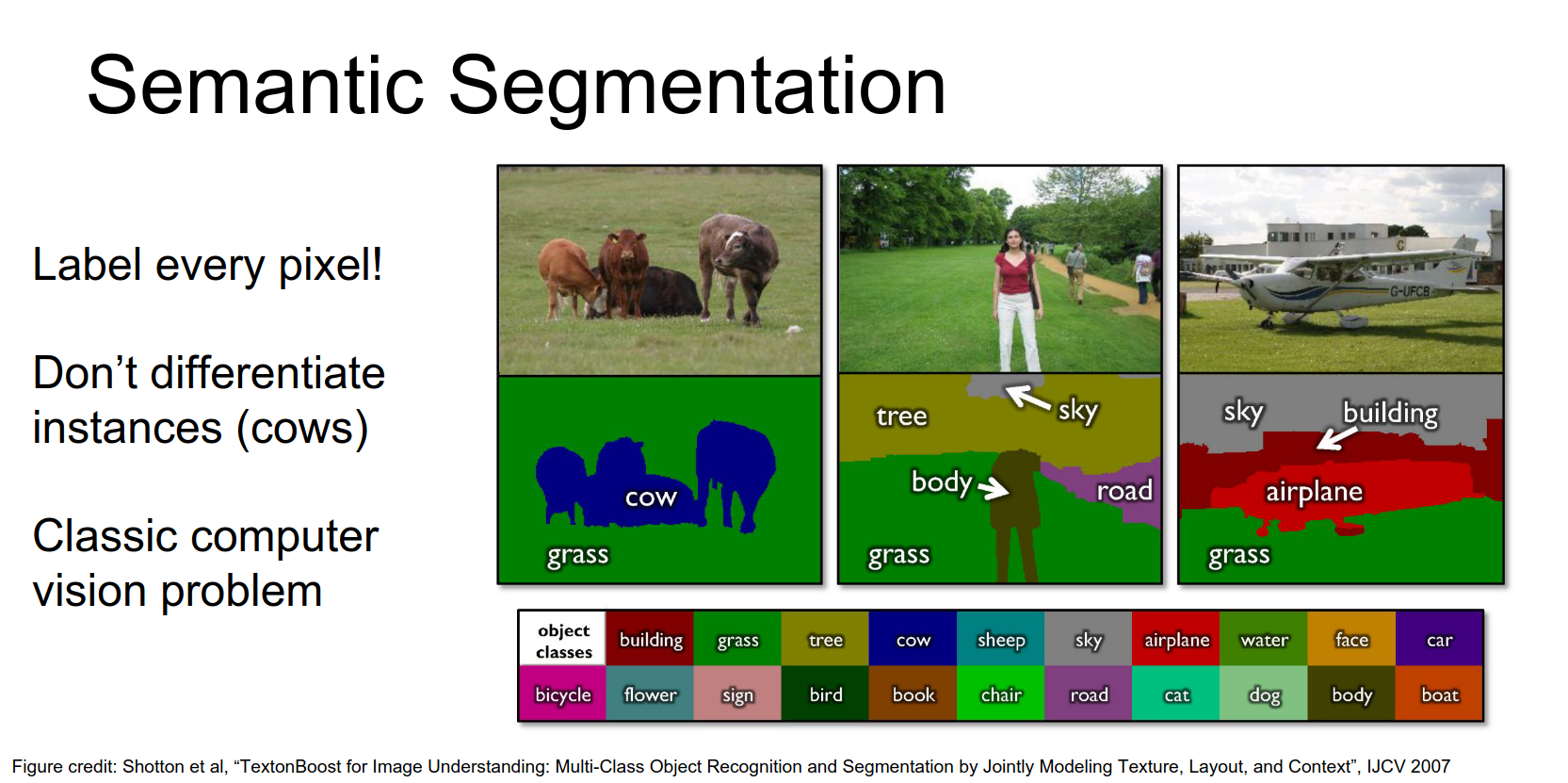
Semantic Segmentation

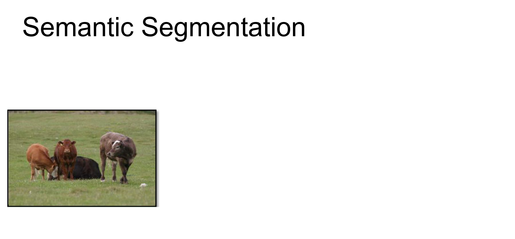
In semantic segmentation, we want to label every pixel in the image with a class label (e.g., cow, grass, sky). We do not distinguish between different instances of the same class.

If there are three cows, all their pixels get the same "cow" label.

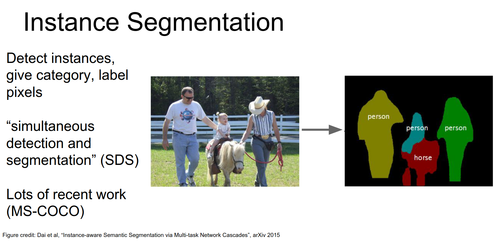
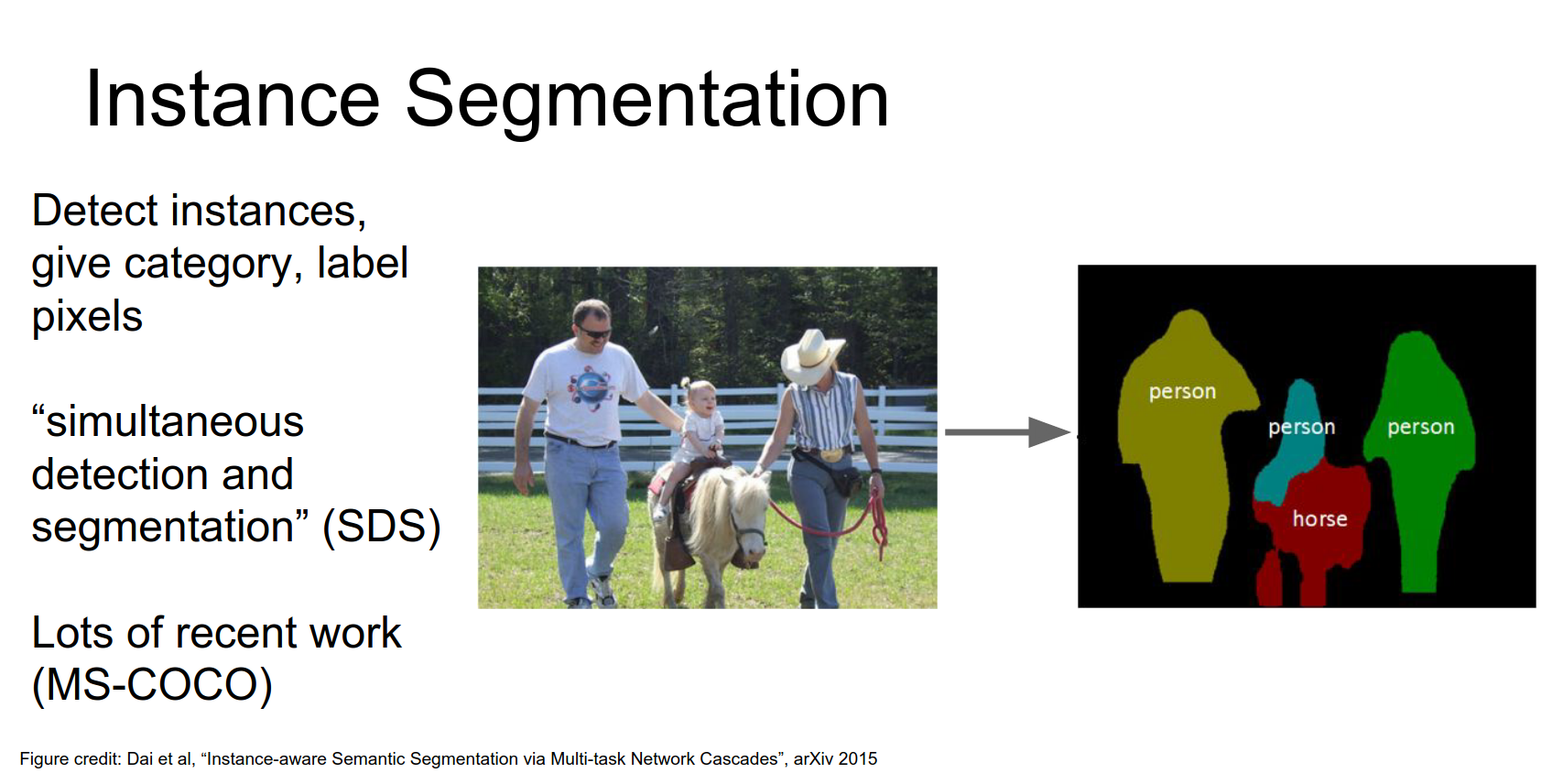
Instance Segmentation

In instance segmentation, we want to detect all instances of objects and segment the pixels belonging to each instance.

Here, we distinguish between the three different people in the image.

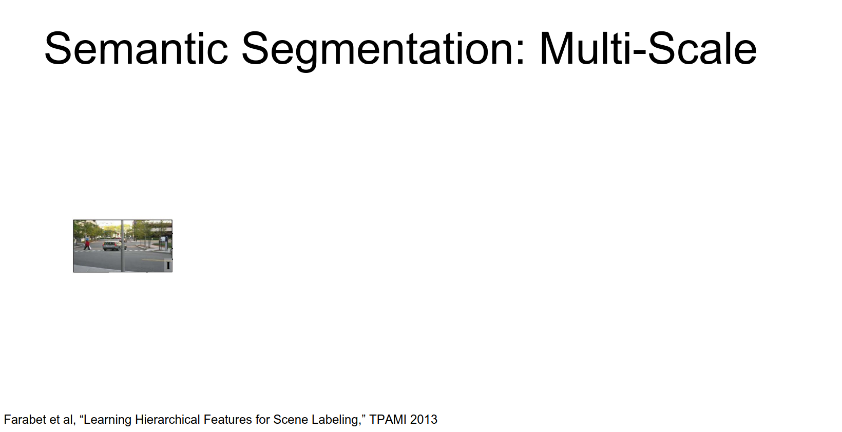
Let's start with Semantic Segmentation.

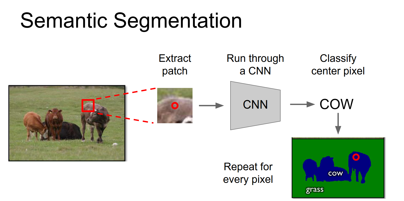
Sliding Window Approach

A simple idea:

1. Take a small patch of the image.
2. Feed it through a CNN to classify the center pixel.
3. Repeat for all pixels.

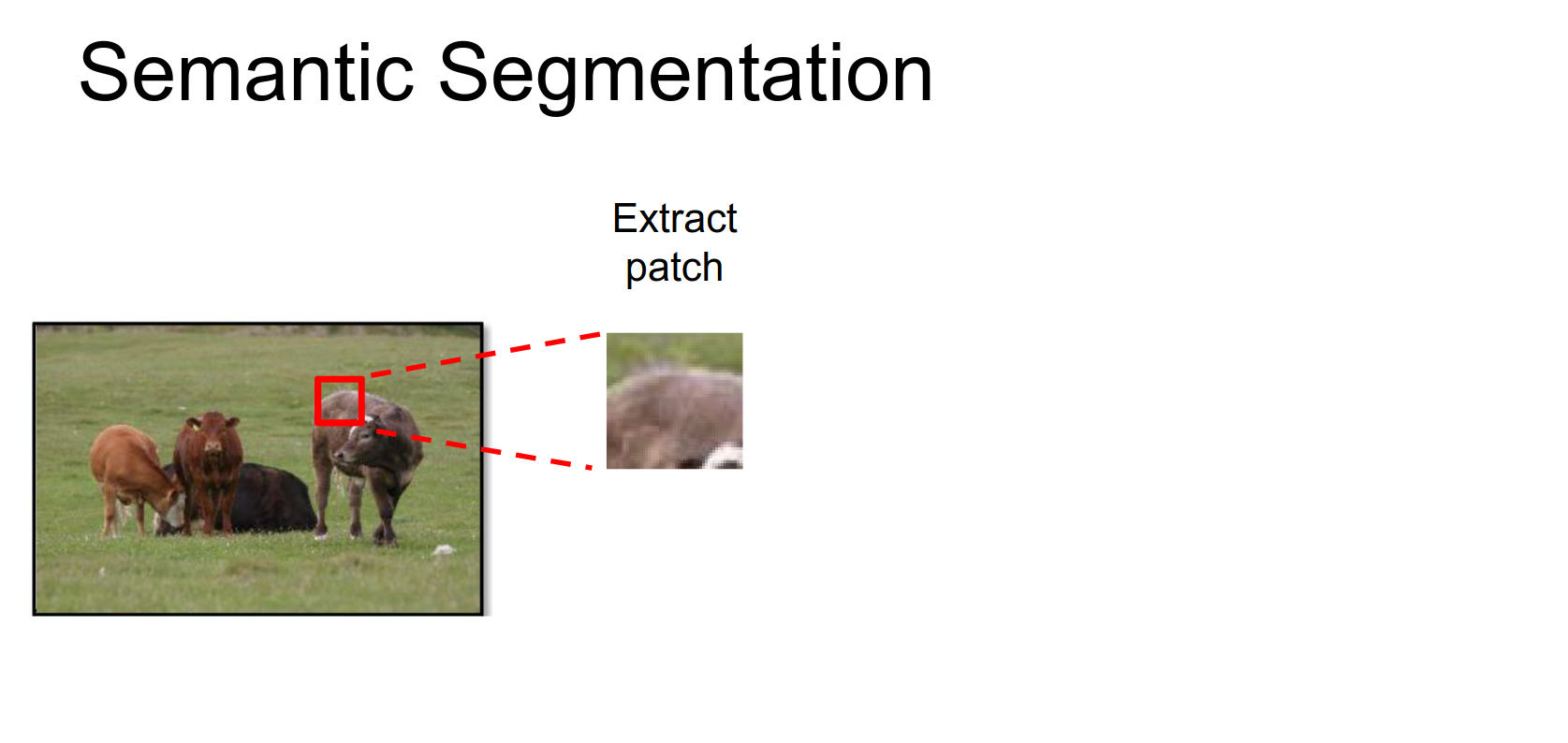
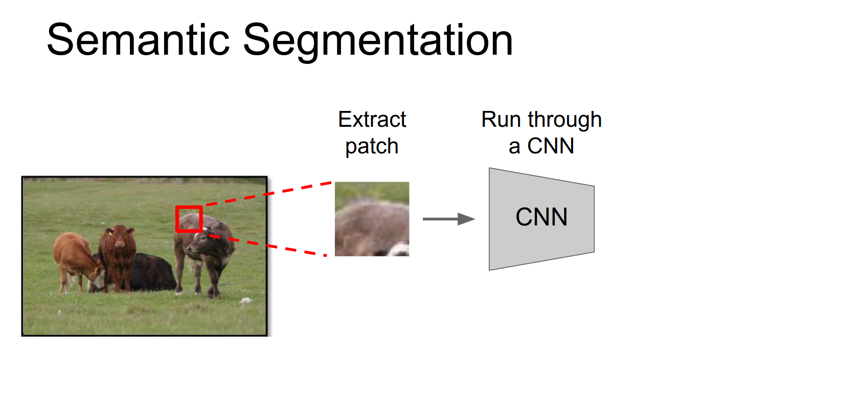
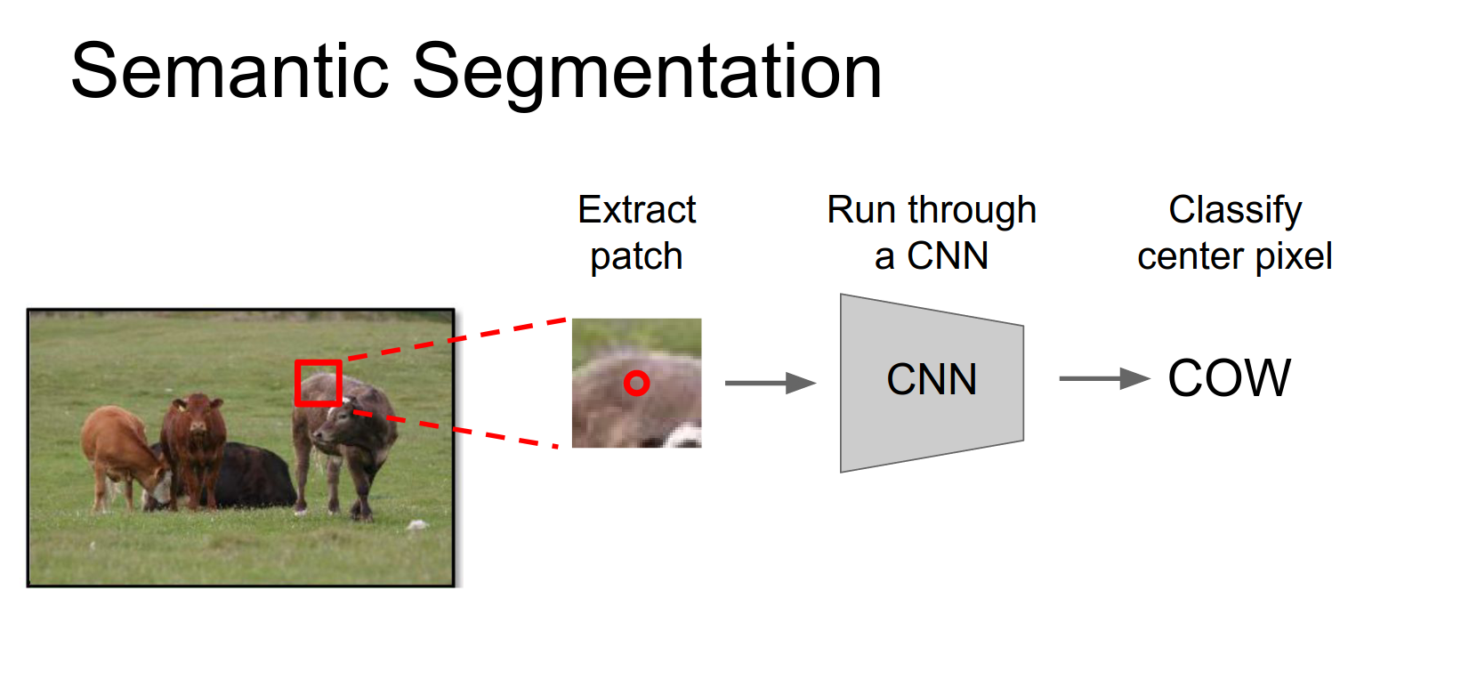
This is very expensive to run independently for every patch.

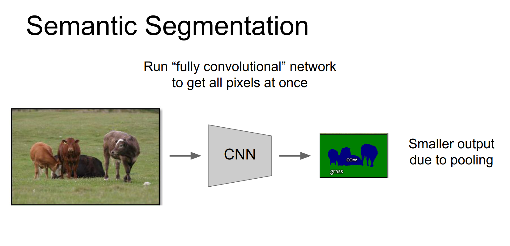
In practice, you can run this fully convolutionally. However, pooling and strided convolutions reduce the spatial resolution, so the output is smaller than the input.

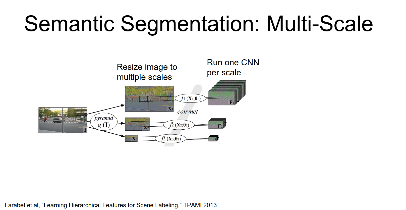
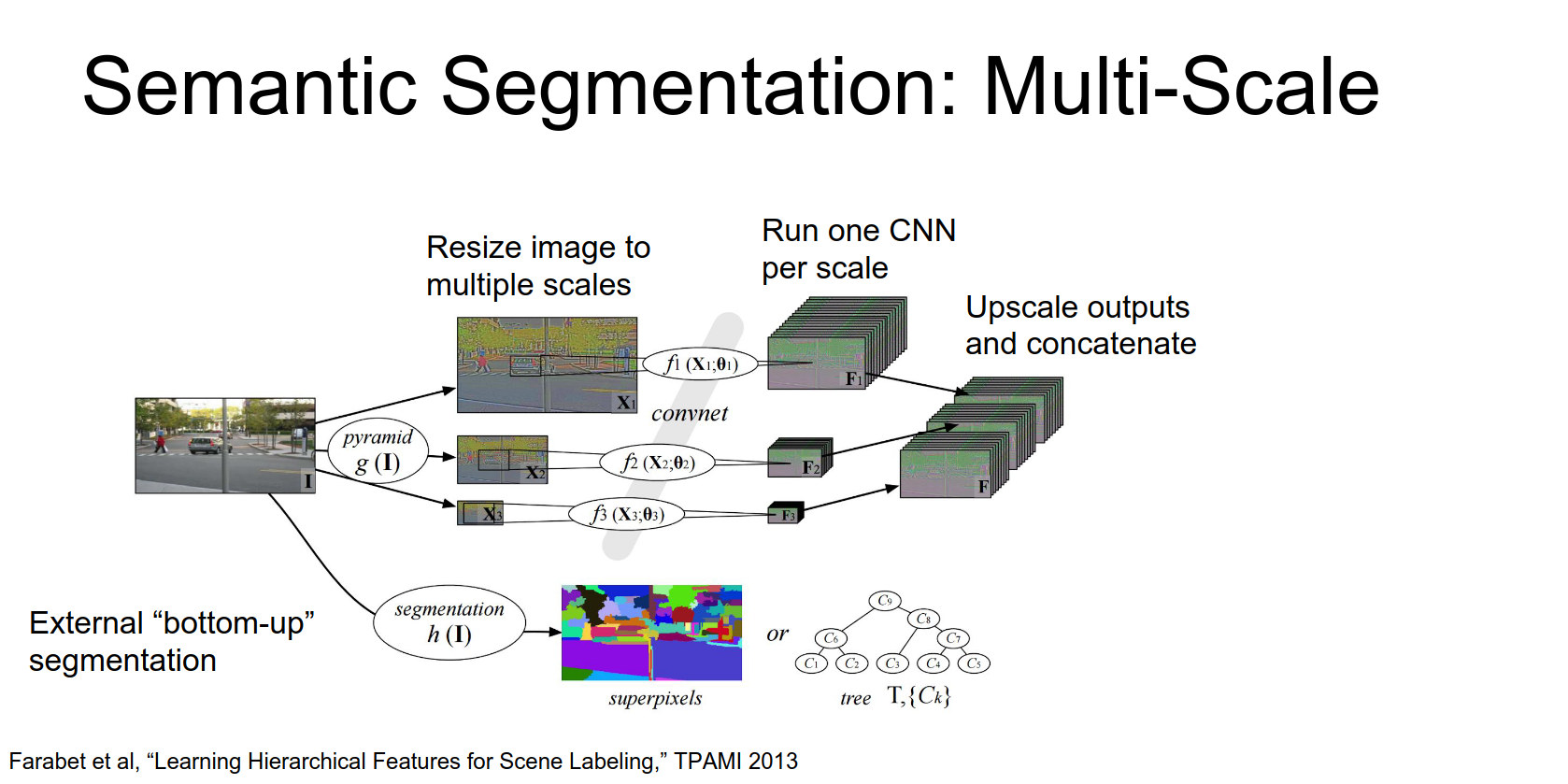
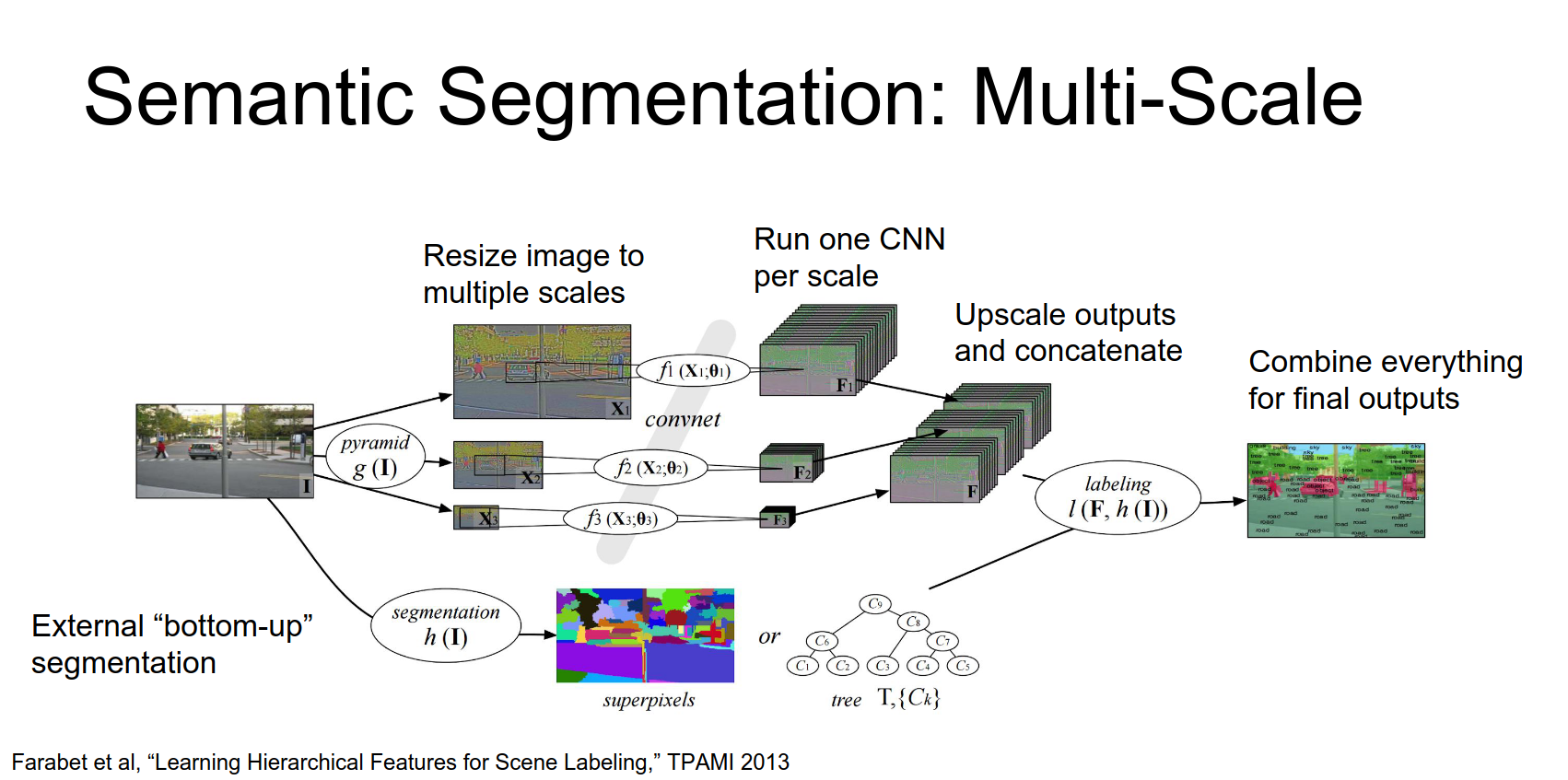
Multi-Scale Testing

To improve performance, people use image pyramids.

1. Resize the input image to multiple scales.
2. Run the CNN on each scale.
3. Upsample the outputs and aggregate them.

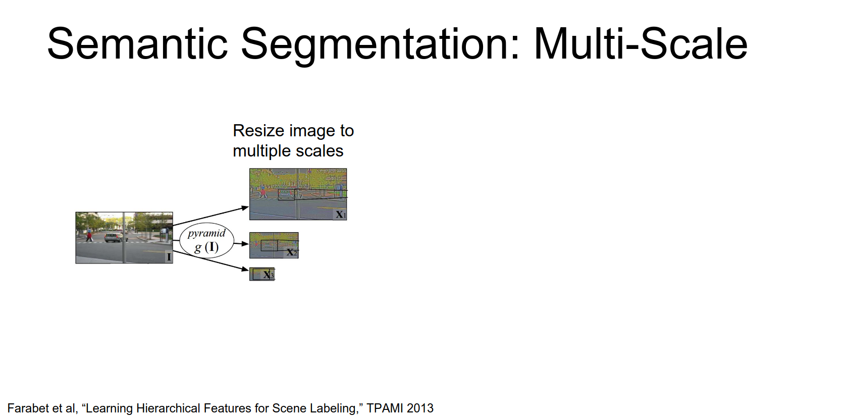
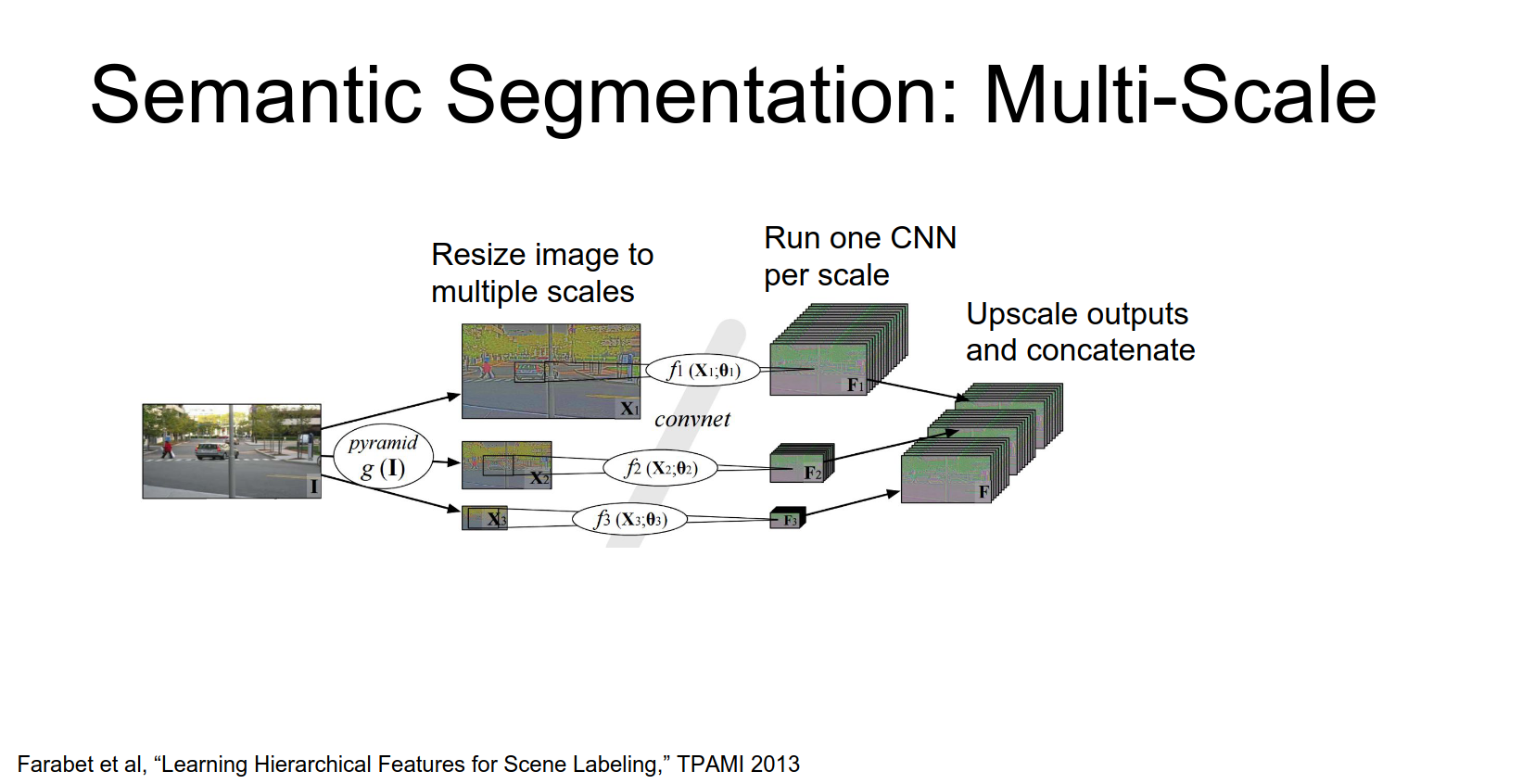
Some approaches (like Farabet et al., 2013) use offline superpixel methods or segmentation trees to refine the output.

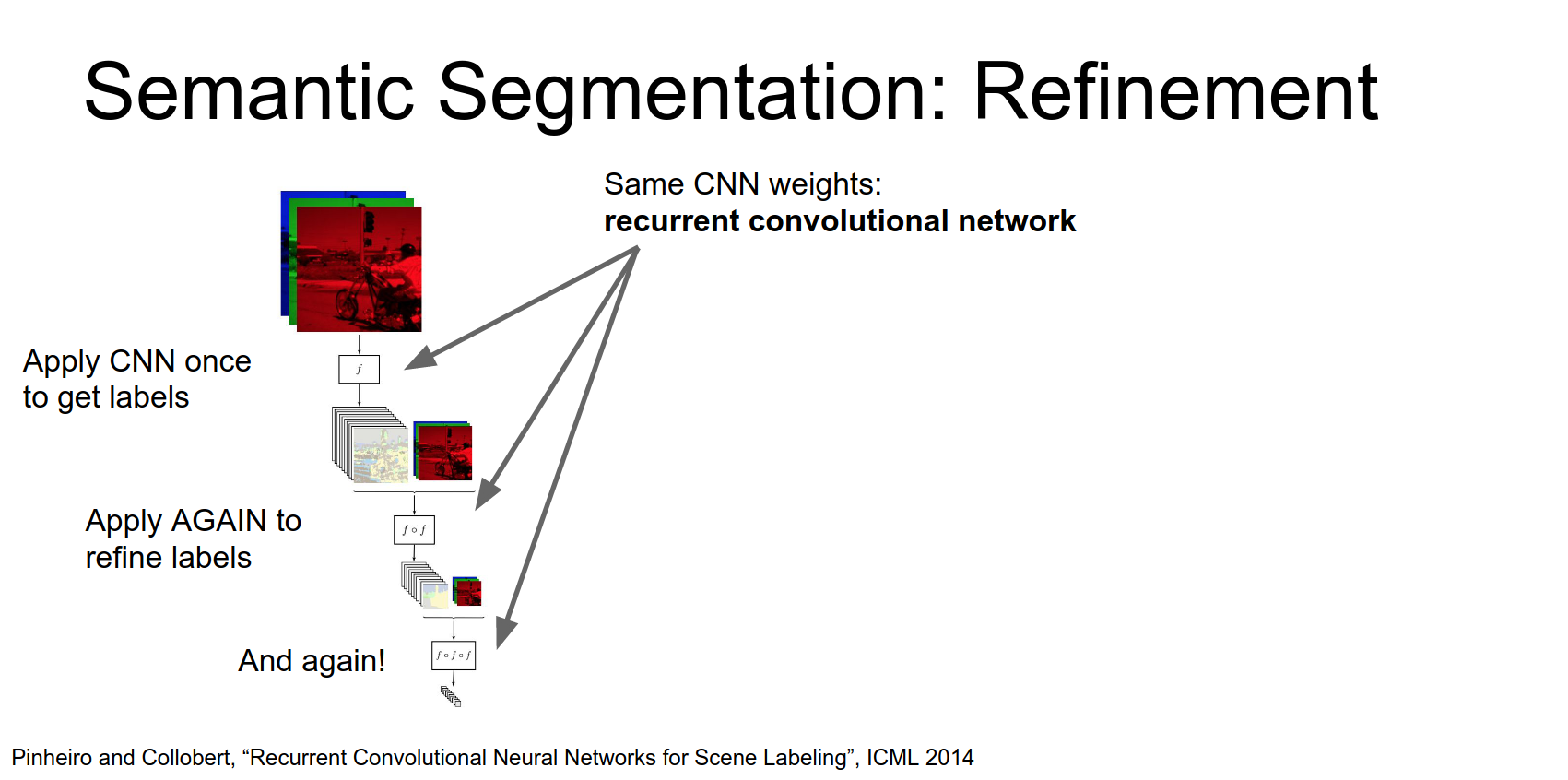
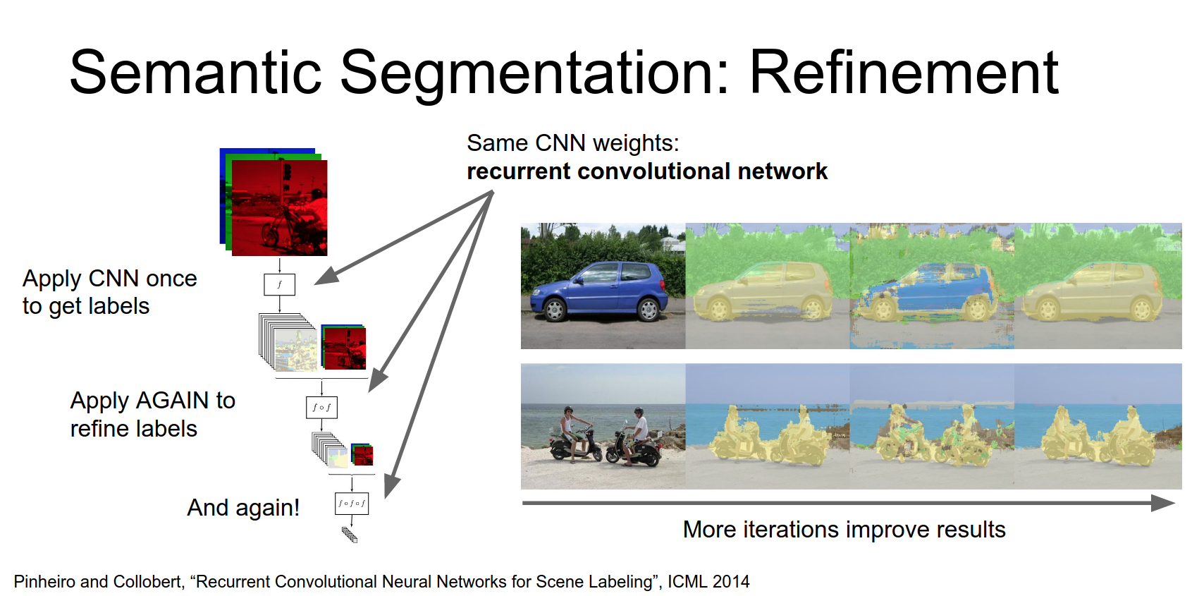
Iterative Refinement

Another idea is to iteratively refine the segmentation.

1. Run the image through a CNN to get a coarse segmentation.
2. Take the coarse output and the downsampled image, and run it through the network again.
3. Repeat.

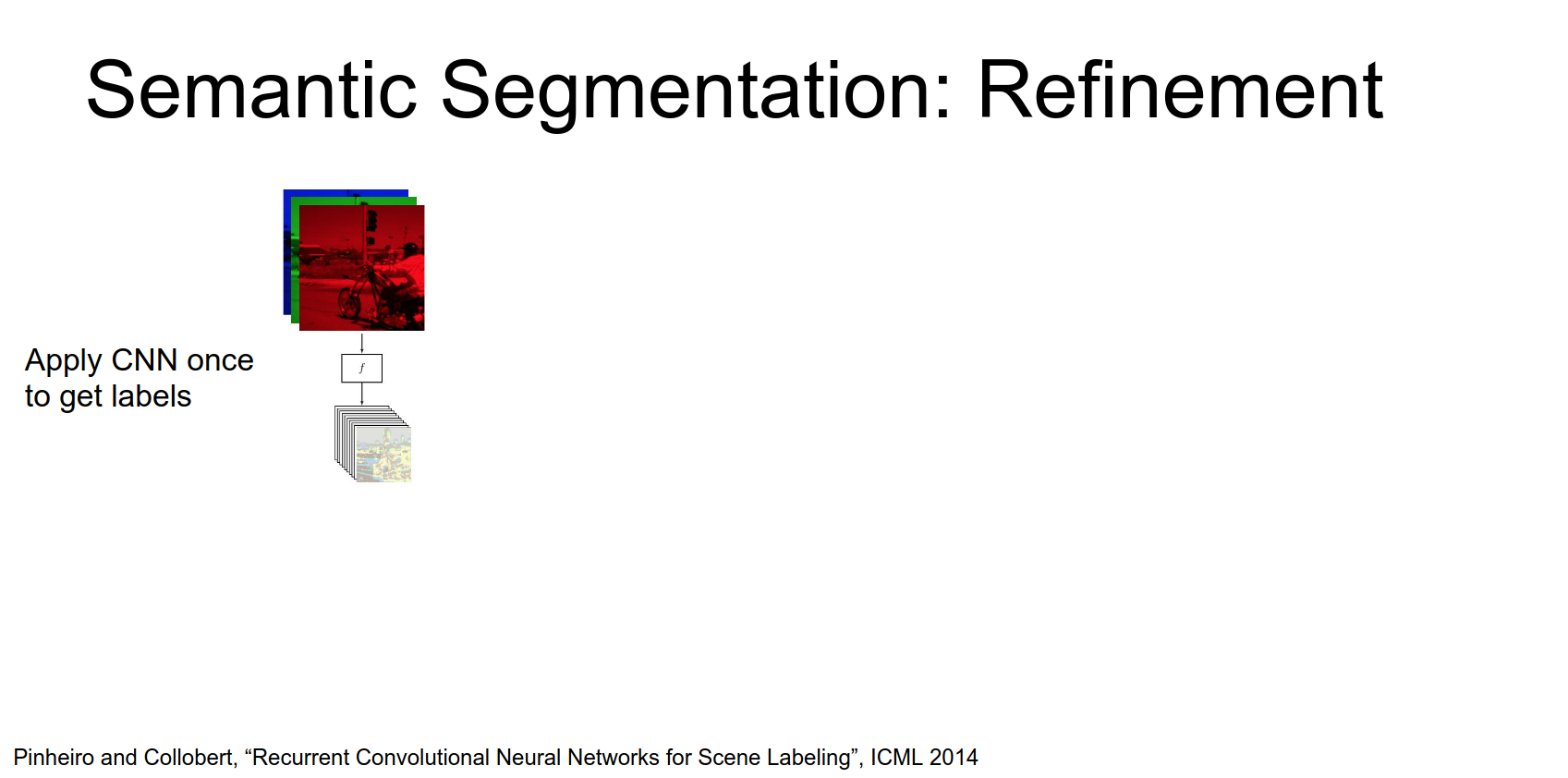
This allows the network to sort of increase its effective receptive field of the output and also to perform more processing on the on the input image.

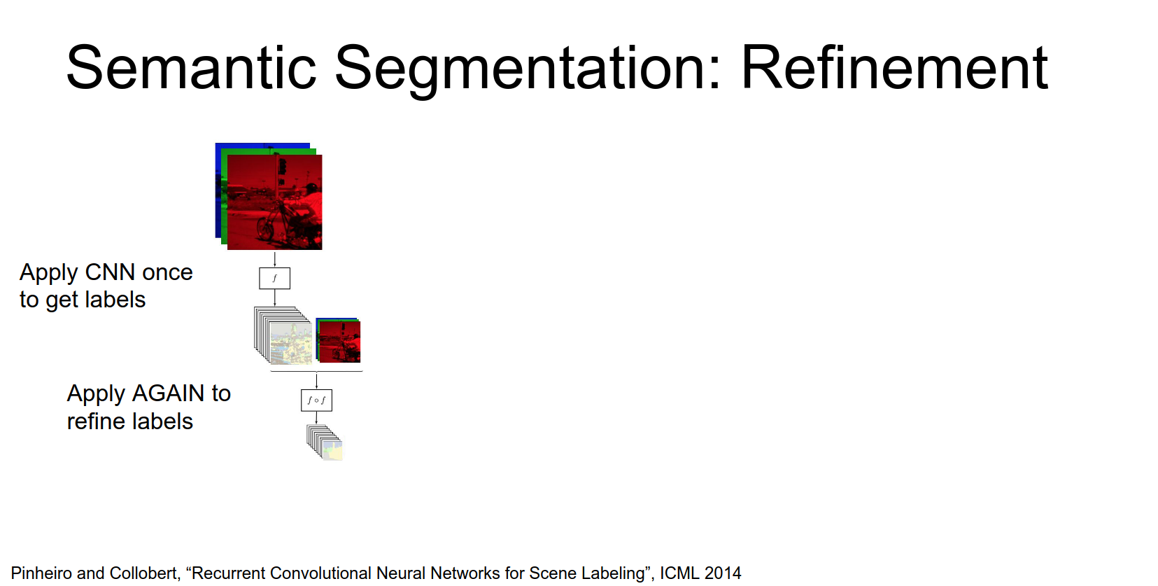
And then we can repeat this process again.

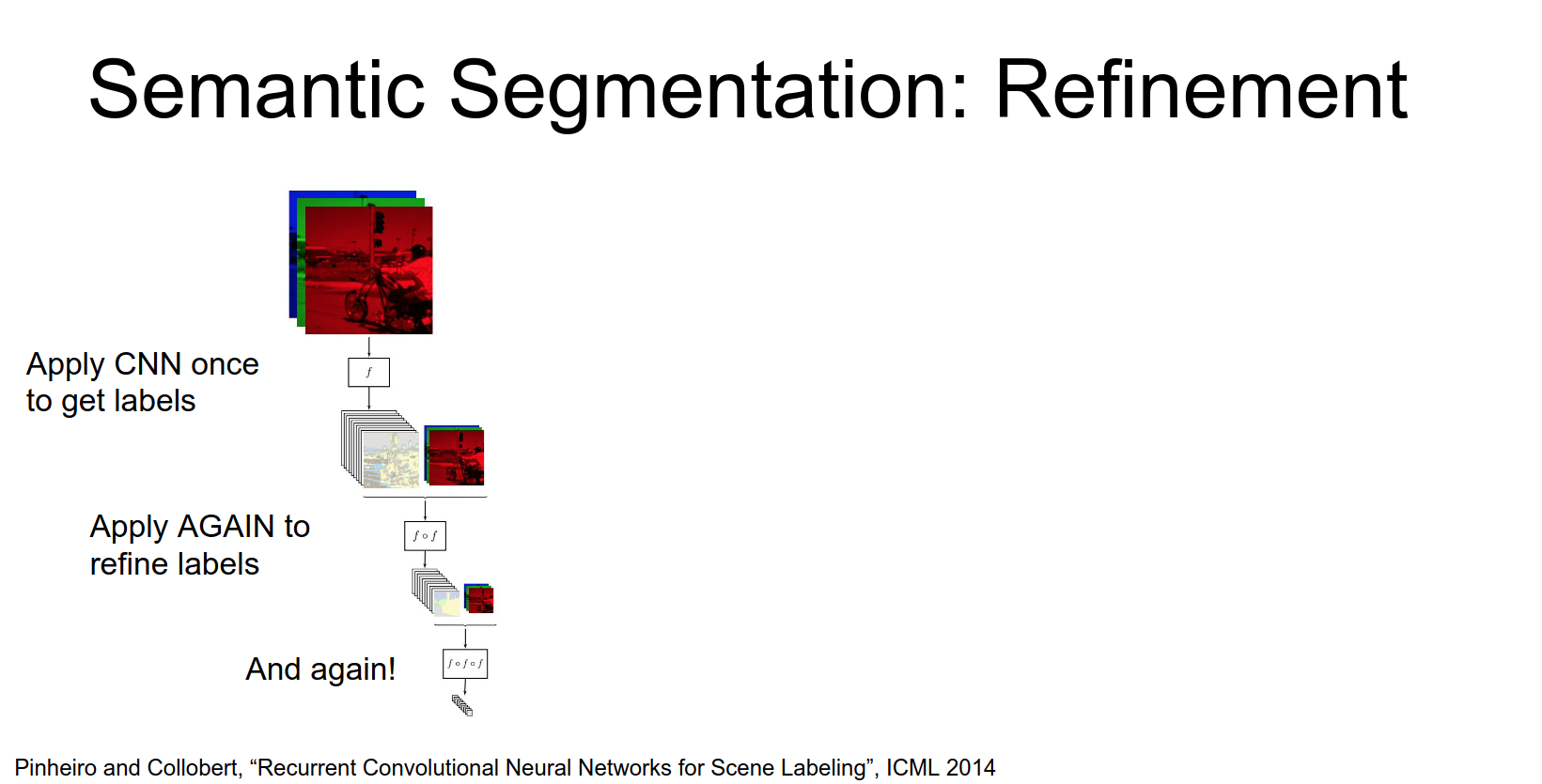
If weights are shared, this is a Recurrent Convolutional Network.

After one iteration you can see that actually there's quite a bit of noise especially around the boundaries of the objects.

But as we run for two and three iterations through this recurrent convolutional network it actually allows the network to clean up a lot of that sort of low-level noise and produce much cleaner and nicer results.

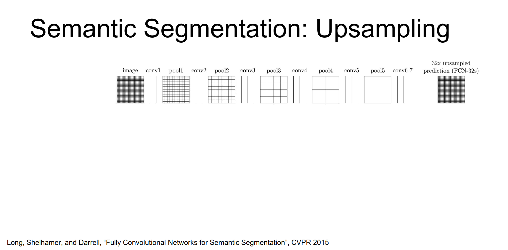
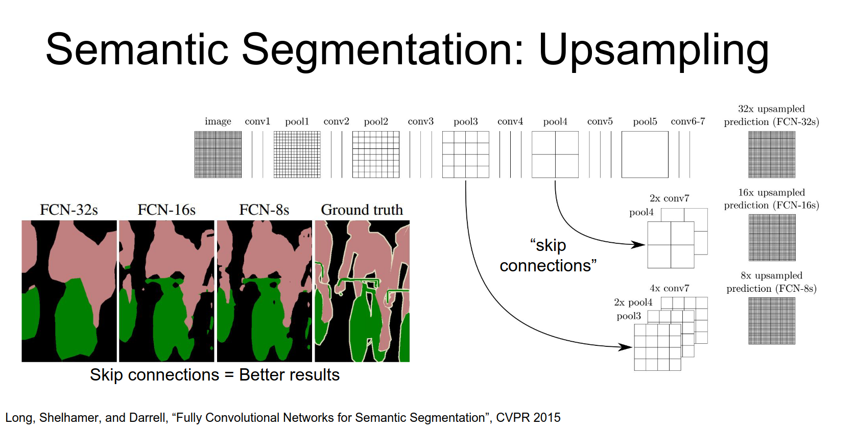
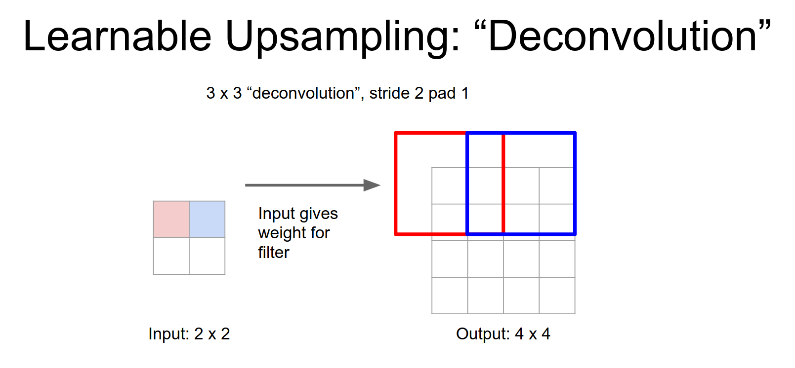
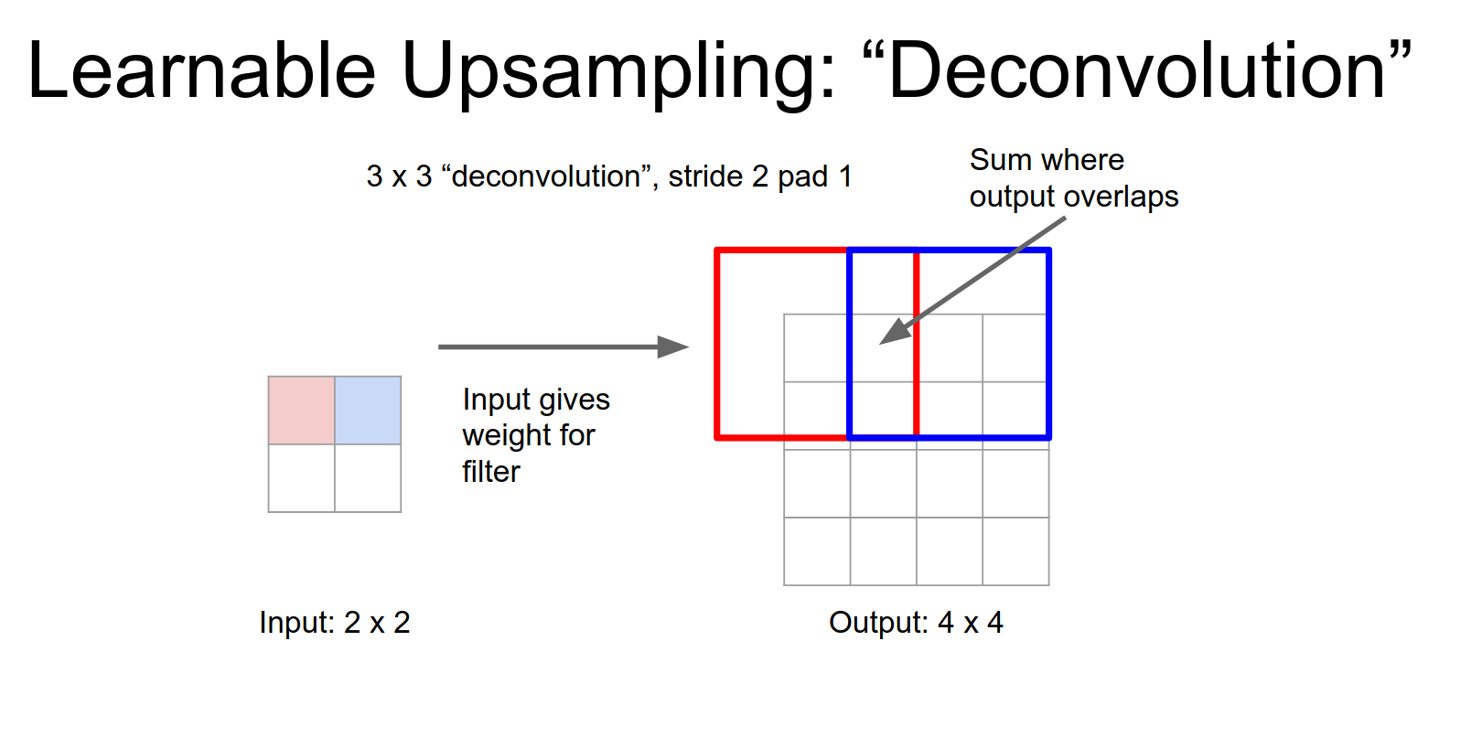
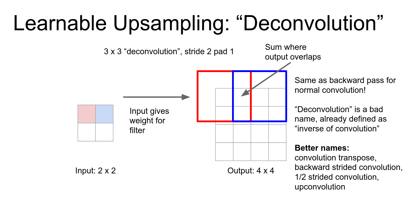
Learnable Upsampling

A famous paper from Berkeley (Long et al., CVPR 2015) proposed learning the upsampling within the network.

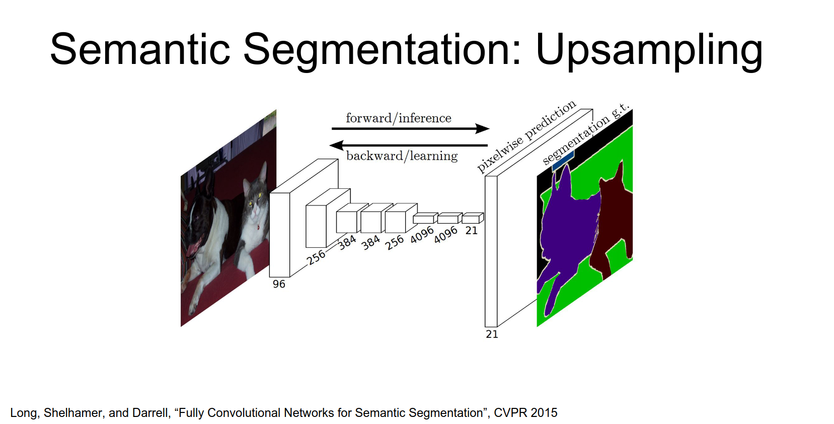
Instead of hard-coded upsampling, they add a learnable upsampling layer at the end.

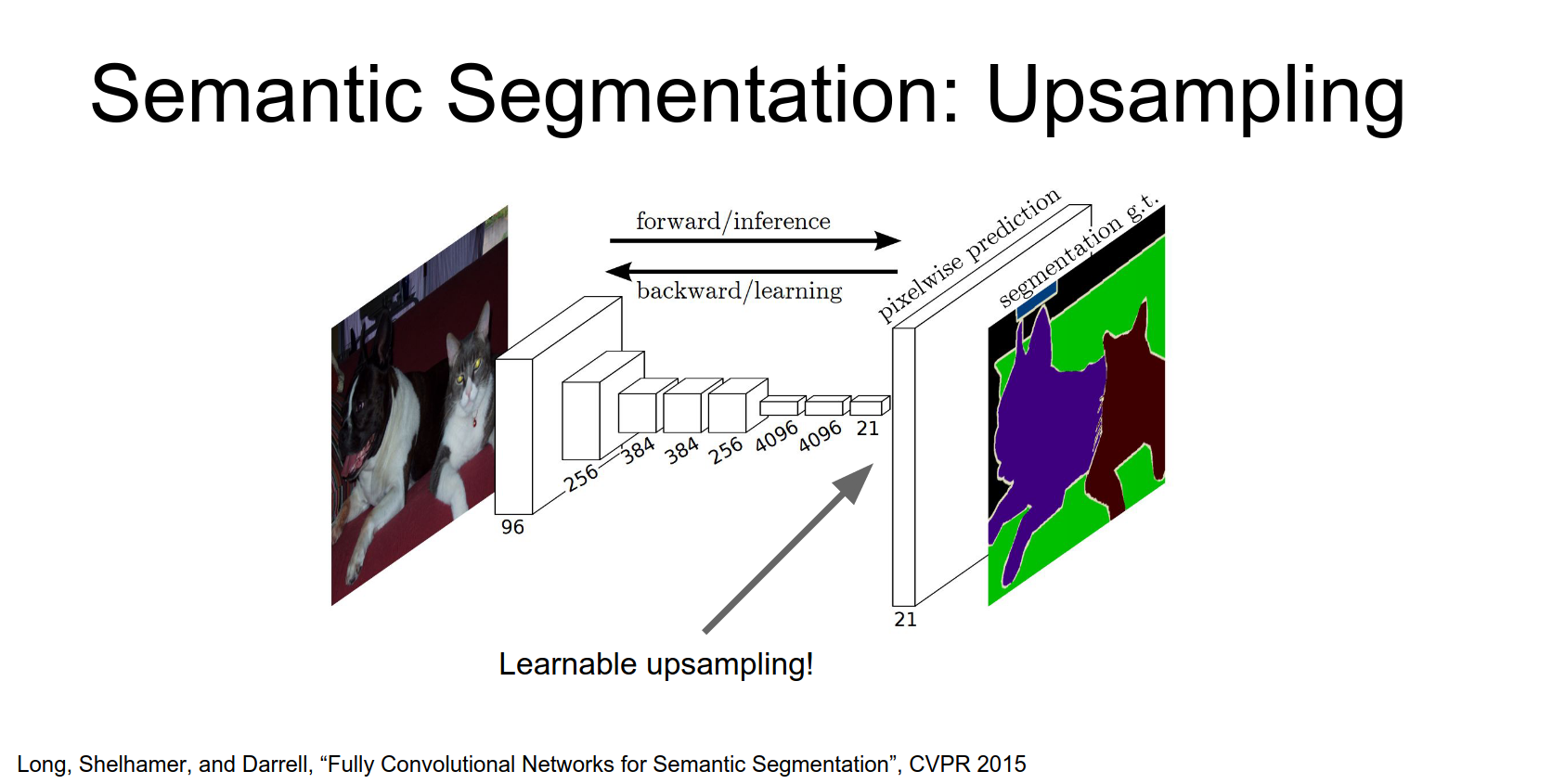
They also use skip connections. They combine features from lower layers (e.g., pool4, pool3) with the final output. Lower layers have smaller receptive fields and capture finer details.

In practice take these different convolutional feature Maps and apply a separate learned up sampling to each of these feature maps, then combine them all to produce the final output.

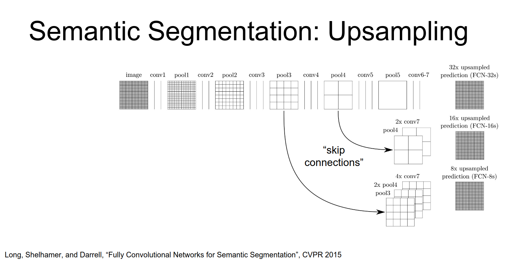
Adding skip connections significantly improves the boundary details.

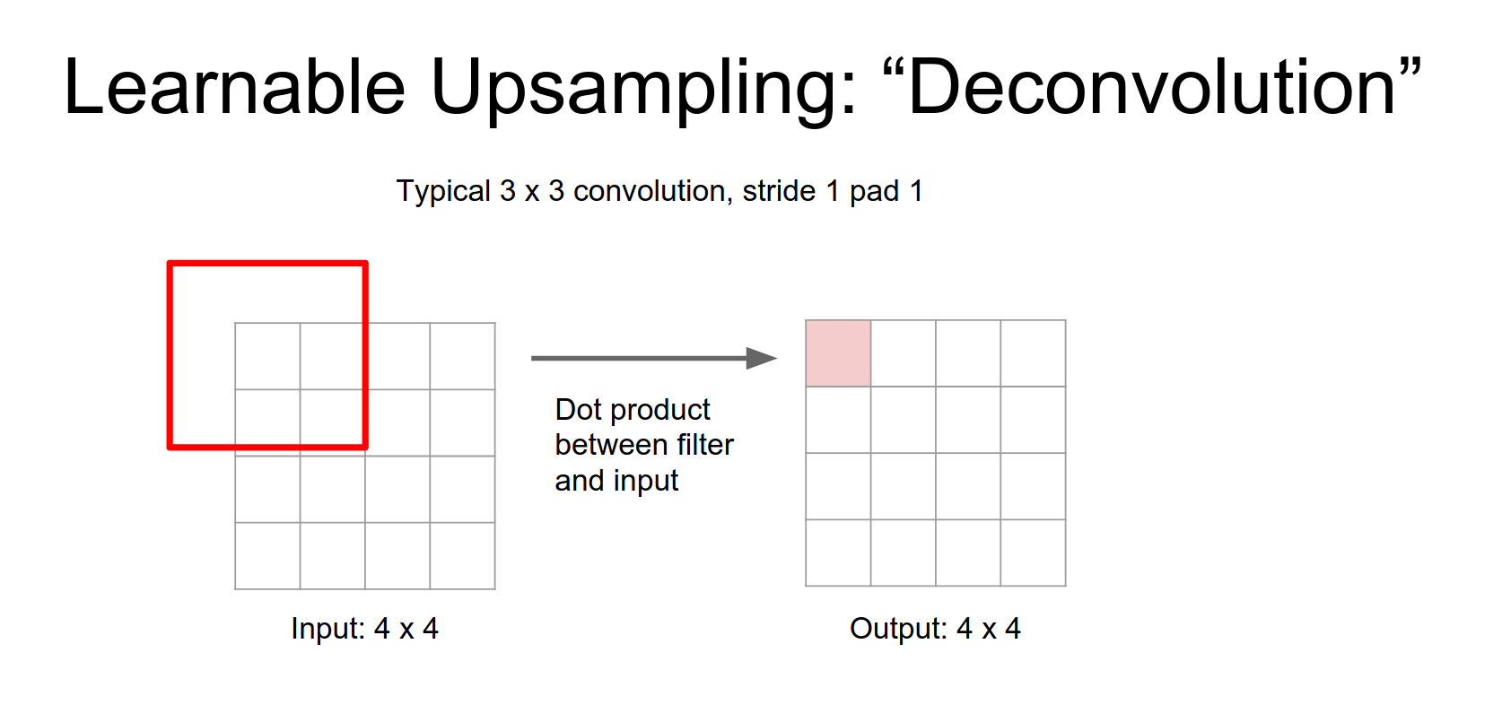
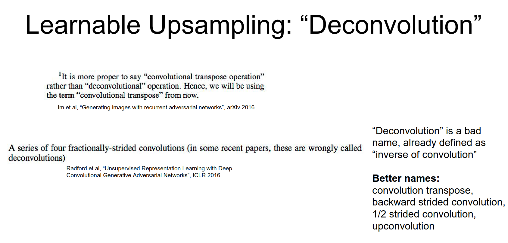
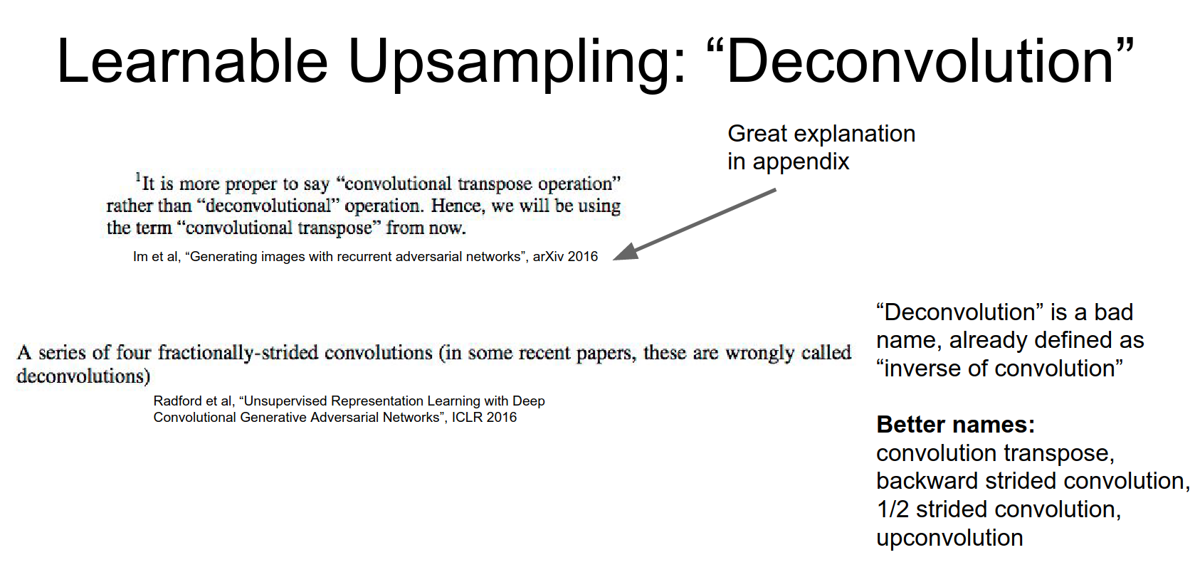
Deconvolution

This learnable upsampling is often called Deconvolution. This is a bad name because it implies the inverse of convolution, which it is not. Better names are Convolution Transpose, Fractionally Strided Convolution, or Up-convolution.

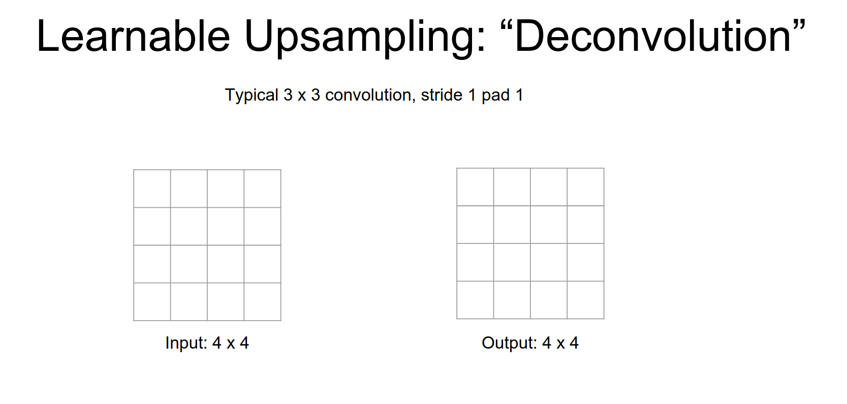
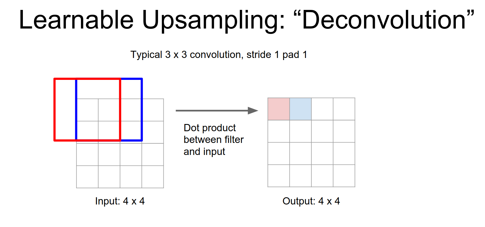
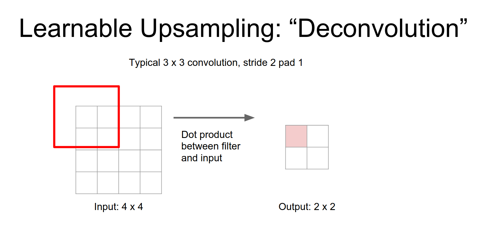
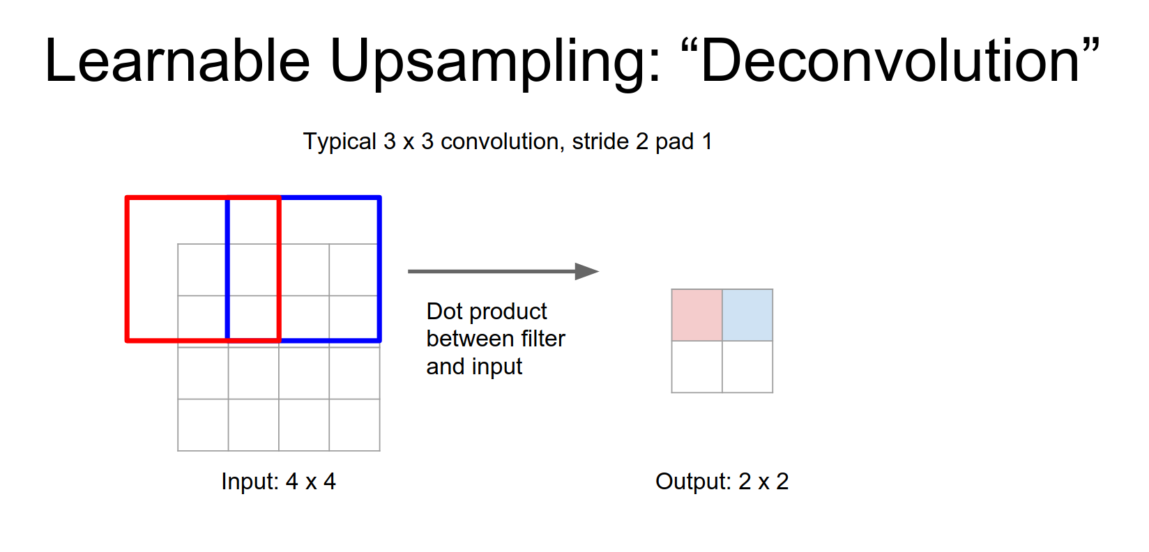
Normal Convolution (Stride 1):

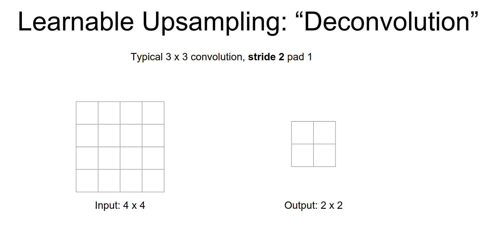
For stride 2 convolution it's a very similar type of idea.

Normal Convolution (Stride 2)

Now our output is going to be a down sampled version a \(2x2\) output for a \(4x4\) input and again it's the same idea.

Deconvolution (Stride 2):

Here, we take a single input value, multiply it by the filter weights, and place the result in the output.

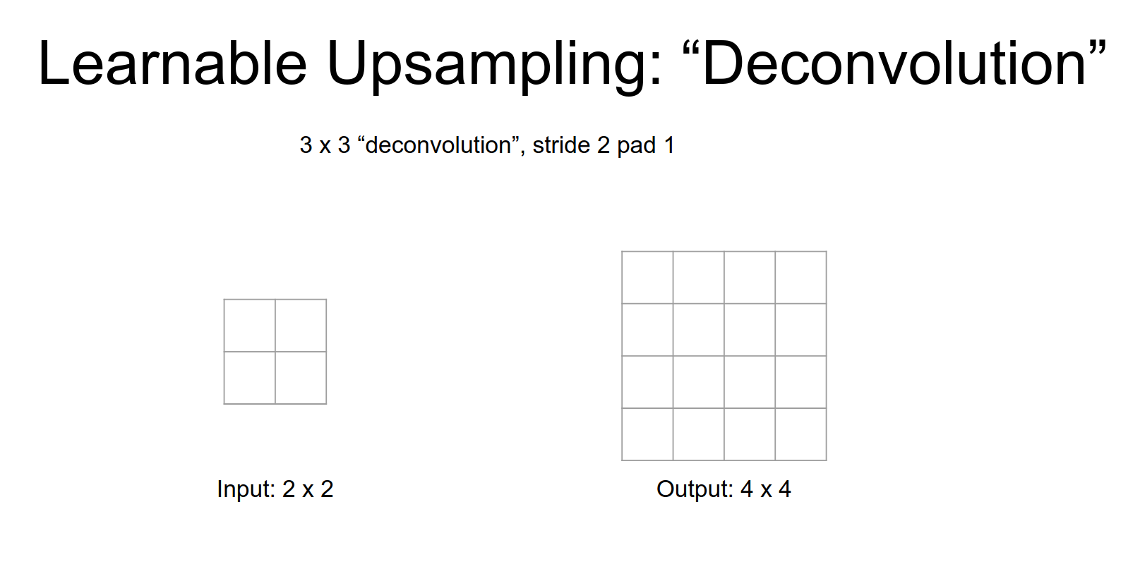
This is a little bit weird, in a normal convolution you have your \(3x3\) filter and you take dot products and the input. But here you have to image taking \(3x3\) filter just copying it over to the output.

The only difference is that, the weights - like this one scalar value of the weight - in your input gives you a weight, you're going to re-weight that filter when you stamp it down into the output.

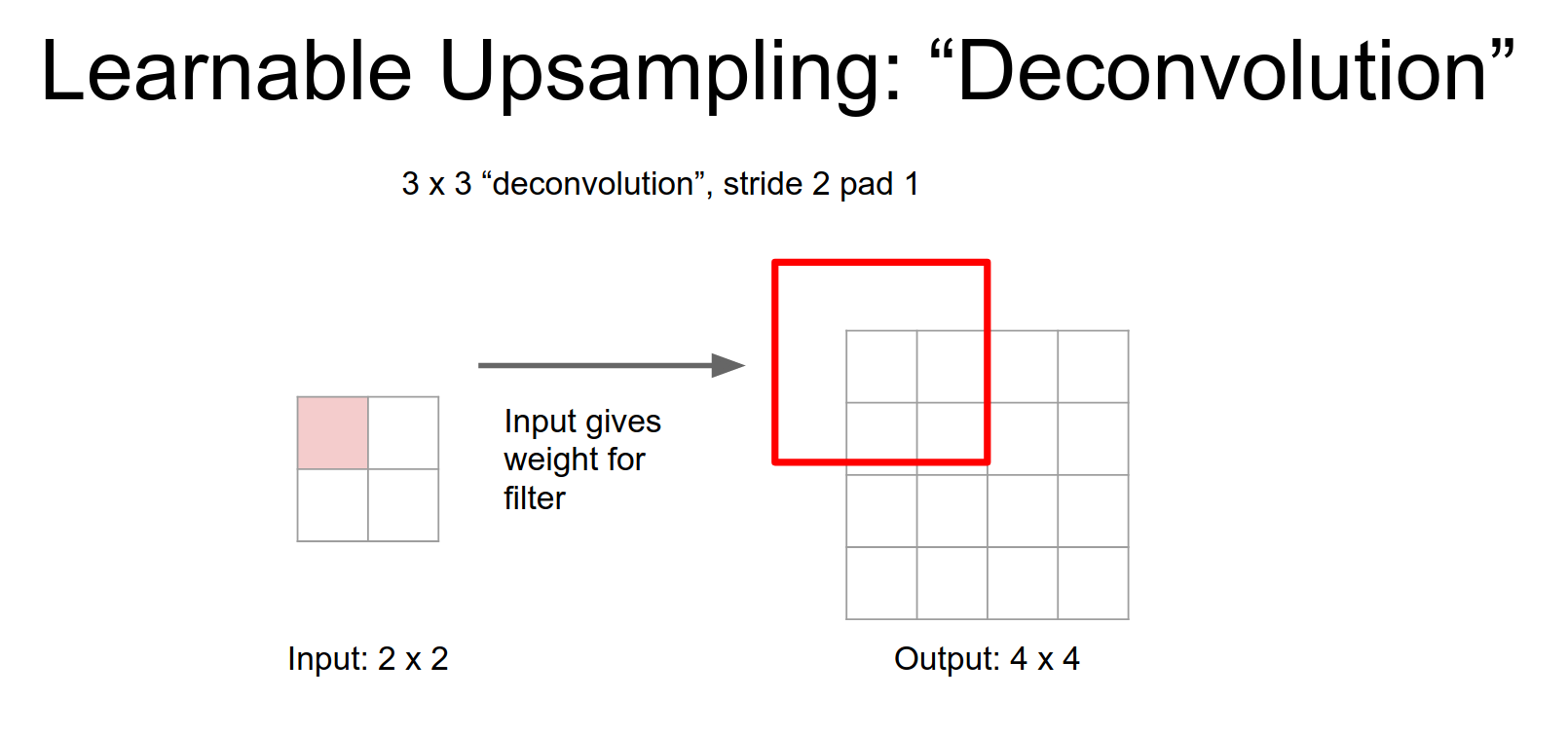
When we stride, we move by the stride in the output. Overlapping regions are summed.

This allows you to learn and up sampling inside the network.

This operation is mathematically equivalent to the backward pass of a normal convolution.

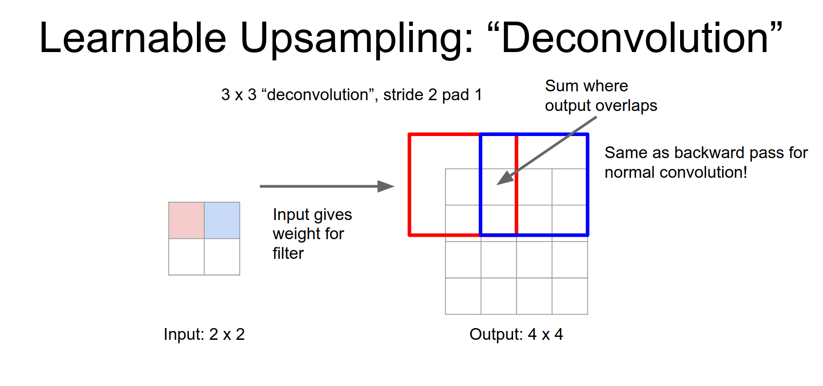
Convolution transpose is much better name.

In practice nobody even thinks to run this thing in a fully patch based mode because that would just be way too slow.

Another trick instead of upsampling is the "shift-and-stitch" method (running the network on shifted versions of the input), but learnable upsampling is generally cleaner.

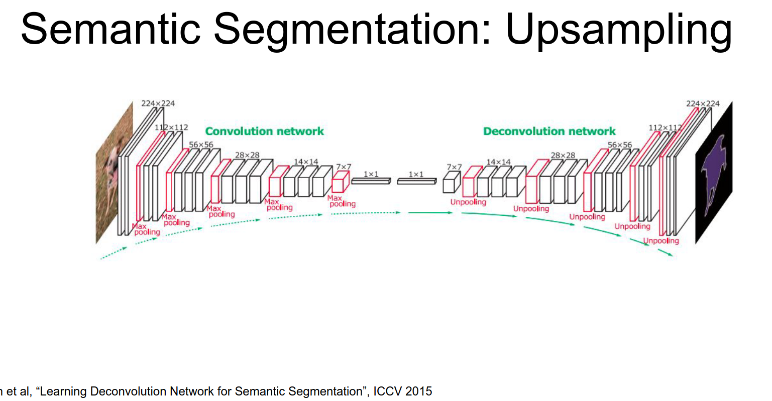
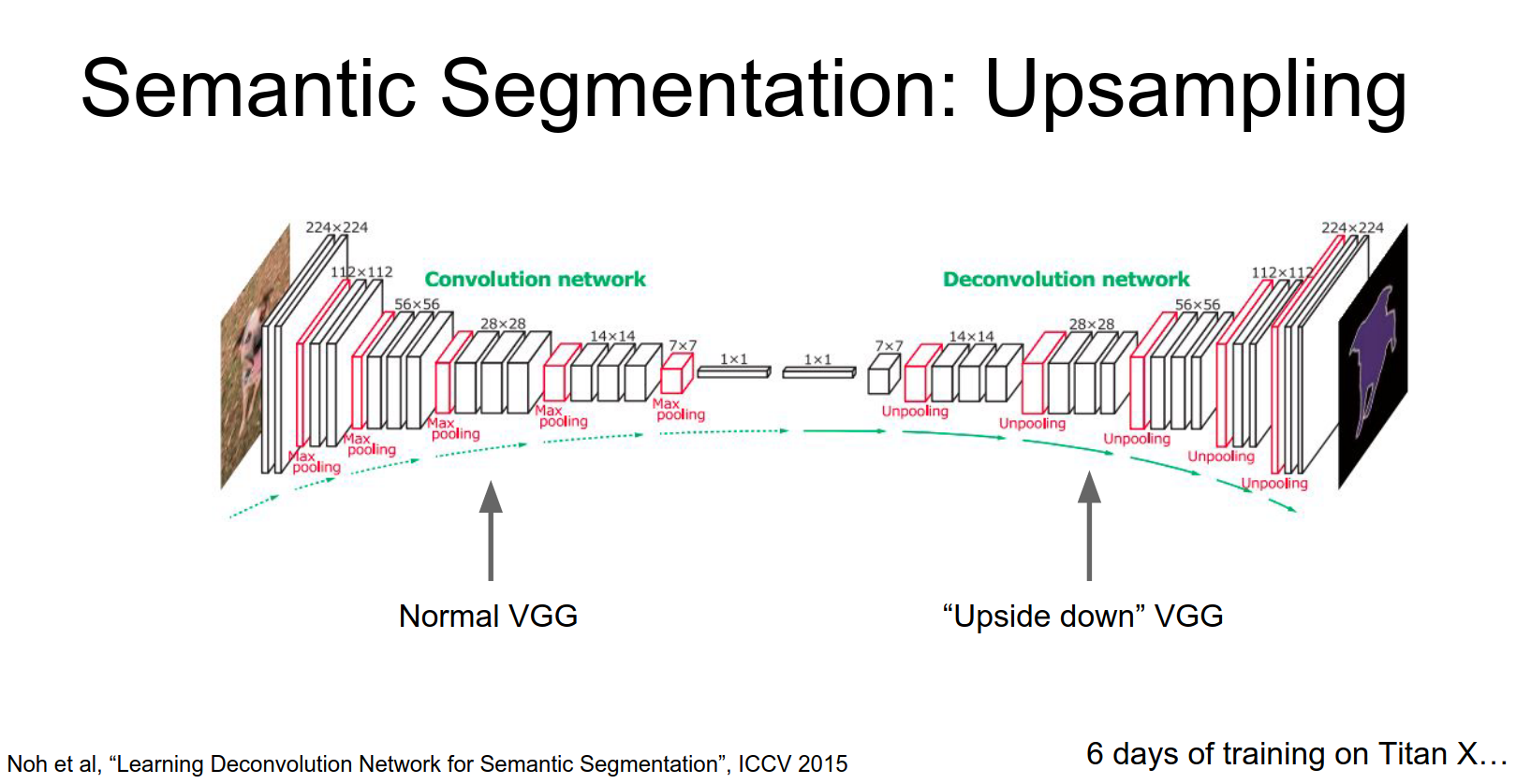
There was also a paper (DeconvNet) that used a symmetric encoder-decoder architecture with unpooling and deconvolution layers.

Data: Pascal VOC is a common dataset. LabelMe is a tool for creating segmentation masks.

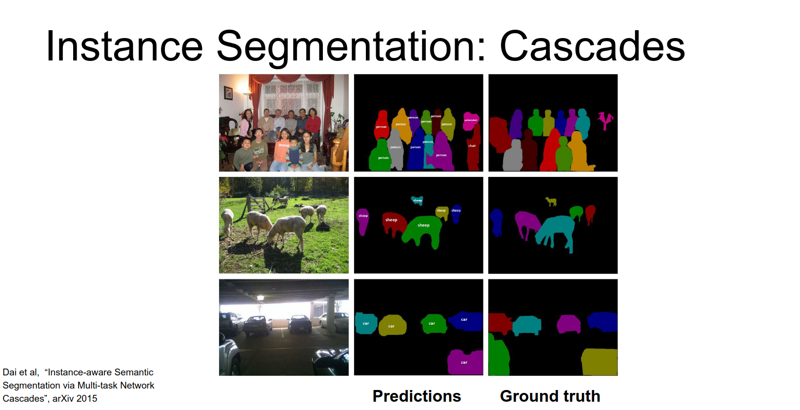
Instance Segmentation

Here we want to distinguish instances.

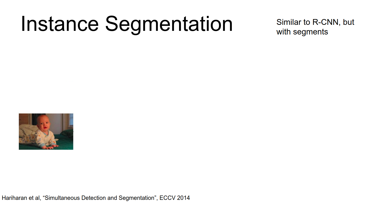
SDS

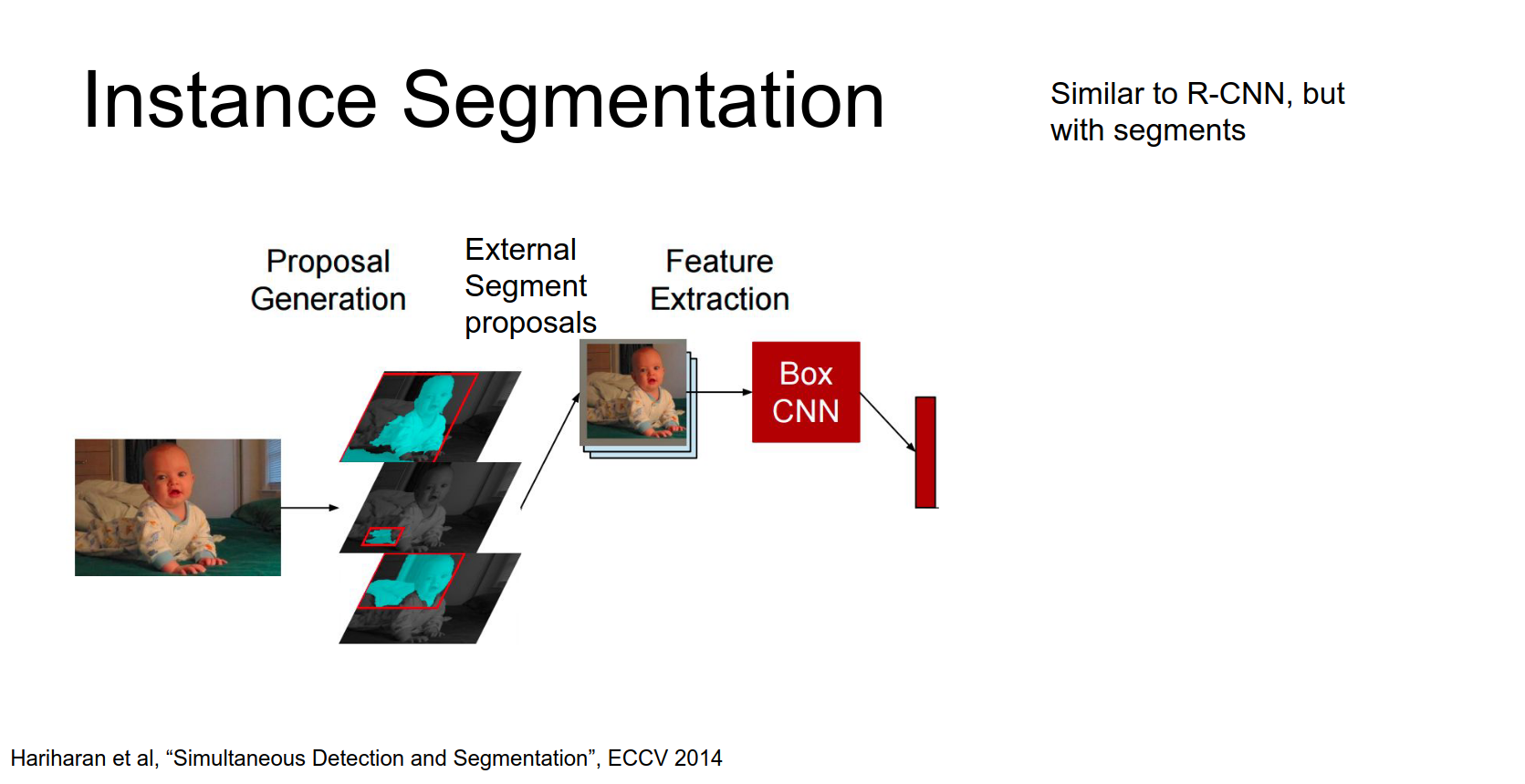
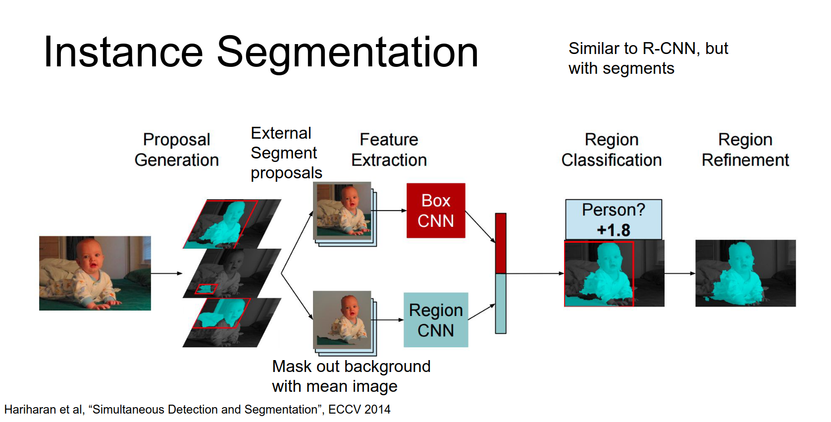
Simultaneous detection and segmentation. This is similar to R-CNN.

If you'll remember in R-CNN we relied on these external region proposals. Turns out that there's other methods for proposing segments instead of boxes.

1. Use a segment proposal method (e.g., MCG) to get candidate segments.
2. Extract a bounding box CNN feature (Box CNN).
3. Extract a region CNN feature (Region CNN) where the background is masked out.
4. Concatenate features and classify.

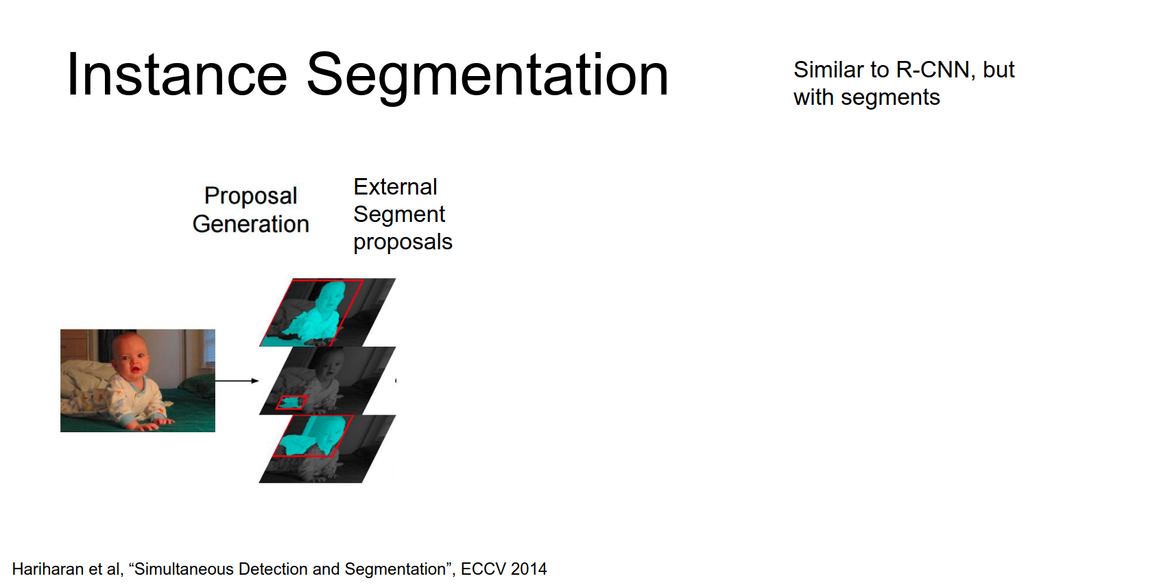
For each of these proposed segments we can extract a bounding box by just fitting a tight box to the segment and then run crop out that chunk of the input image and run it through a box CNN to extract features for that box.

Then in parallel we'll run through a region CNN, so here again we take that relevant that chunk from the input image and crop it out.

But here because we actually have this proposal for the segment, then we're going to mask out the background region using the mean color of the data set.

So this is kind of a hack that lets you take these kind of weird shaped inputs and feed it into a CNN, you just mask out the background part with us with a flat color.

So then they take these masked inputs and run them through a separate region CNN so now we've gotten two different feature vectors one sort of incorporating the whole box and one incorporating only the the proposed foreground pixels.

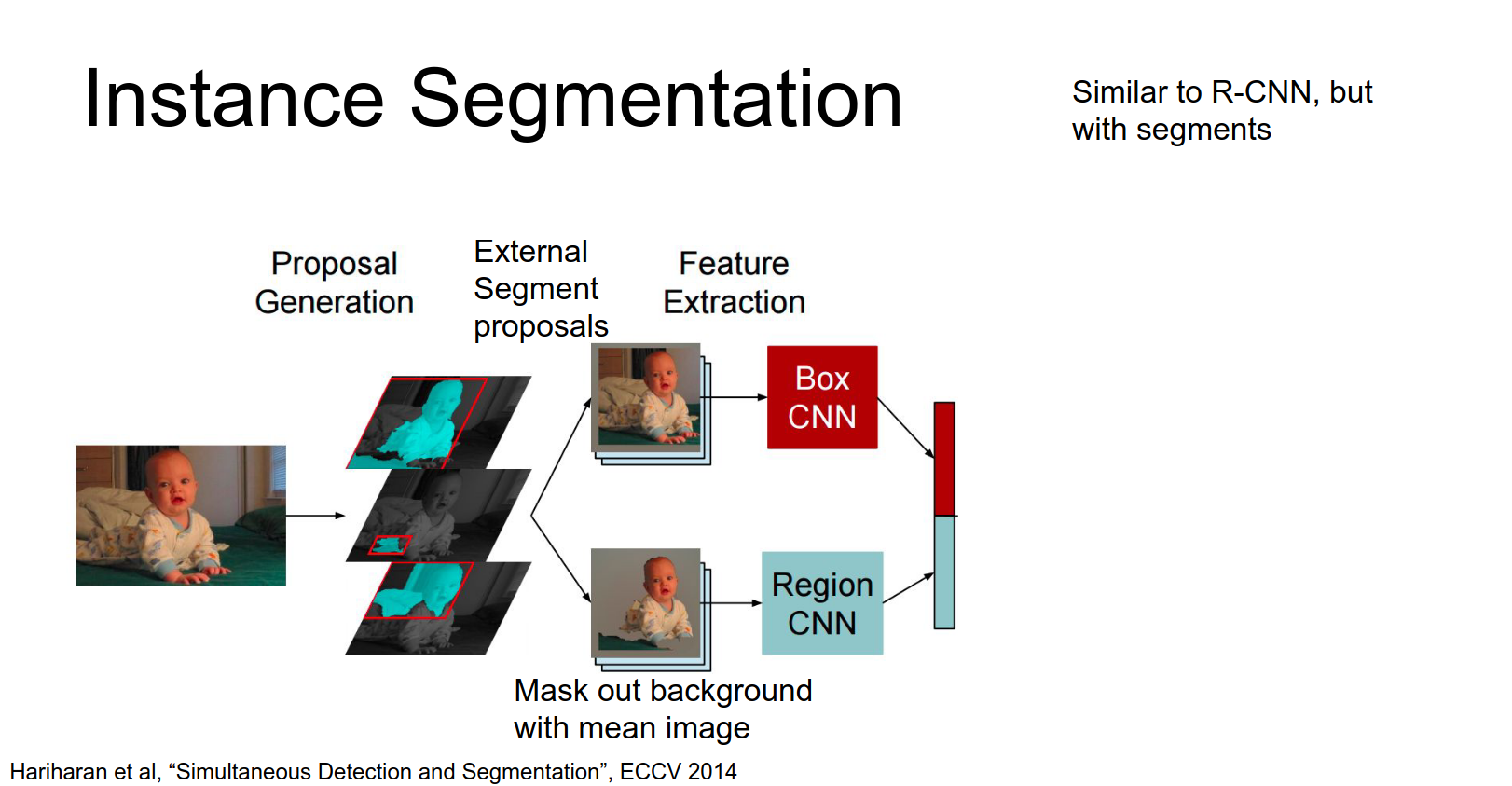
We concatenate these things and then just like in R-CNN we make a classification to decide on what class actually should this segment be.

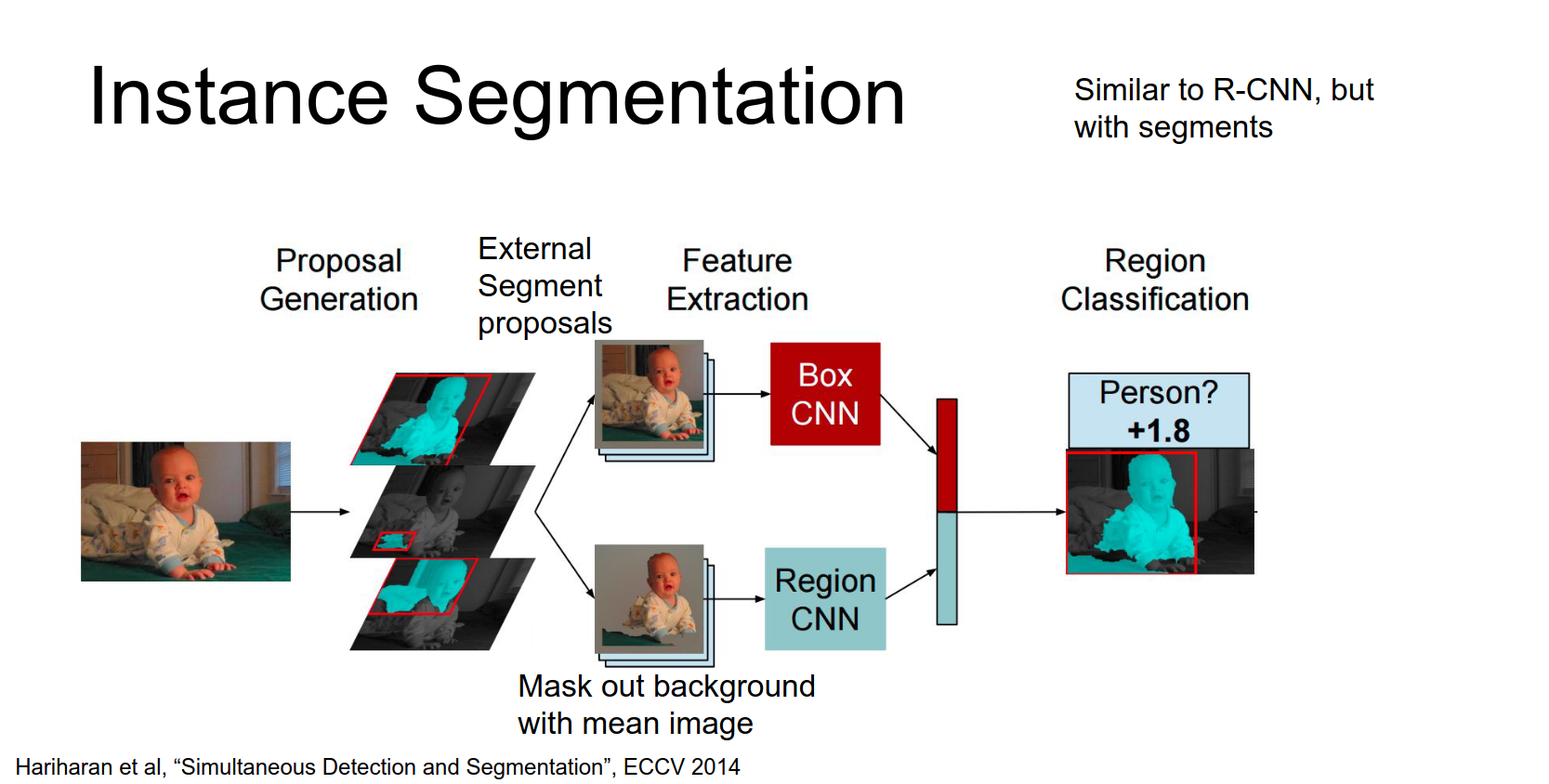
They also perform region refinement.

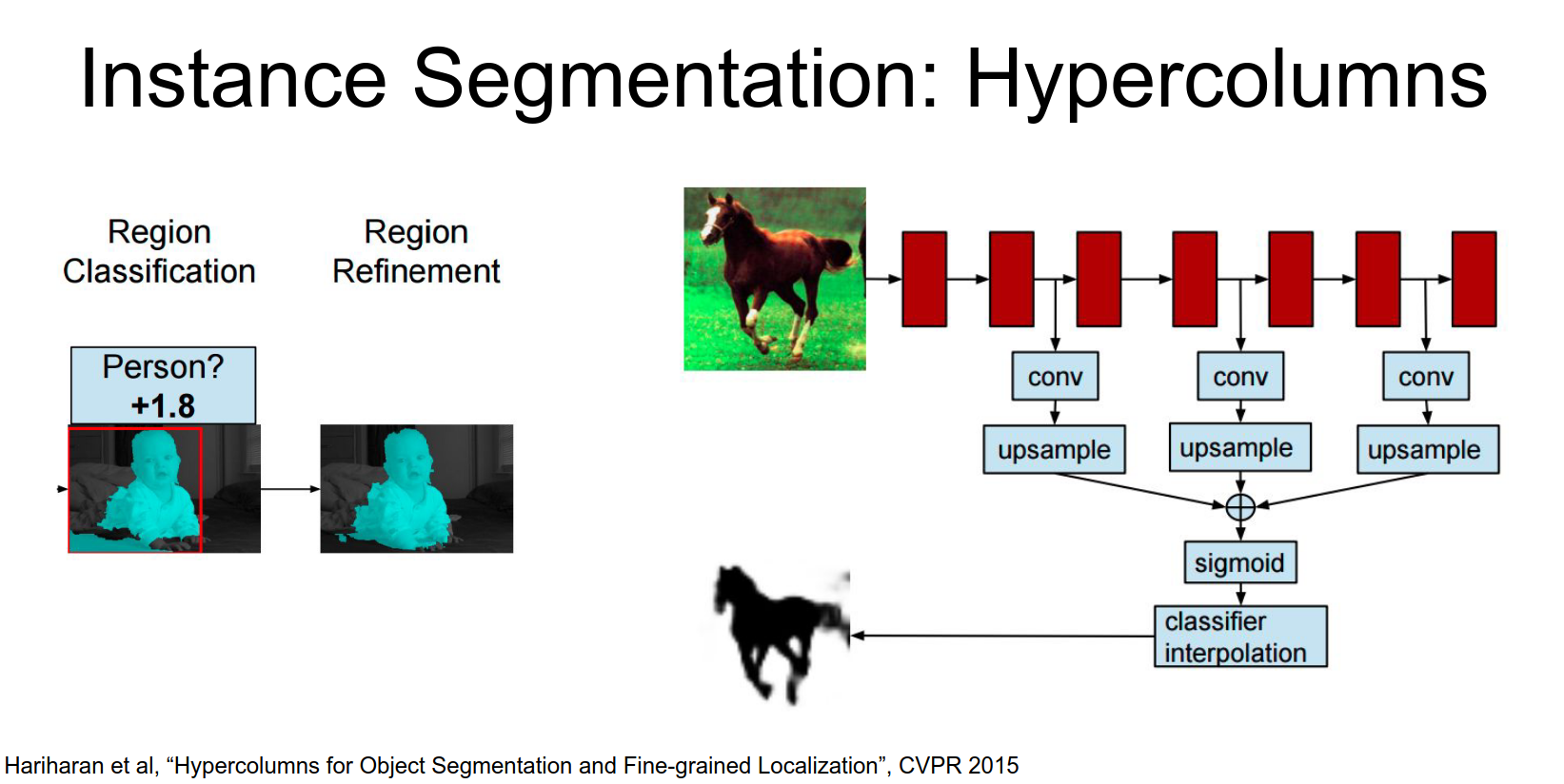
Hypercolumns

A follow-up paper used multi-scale features (Hypercolumns) from AlexNet to refine the segmentation.

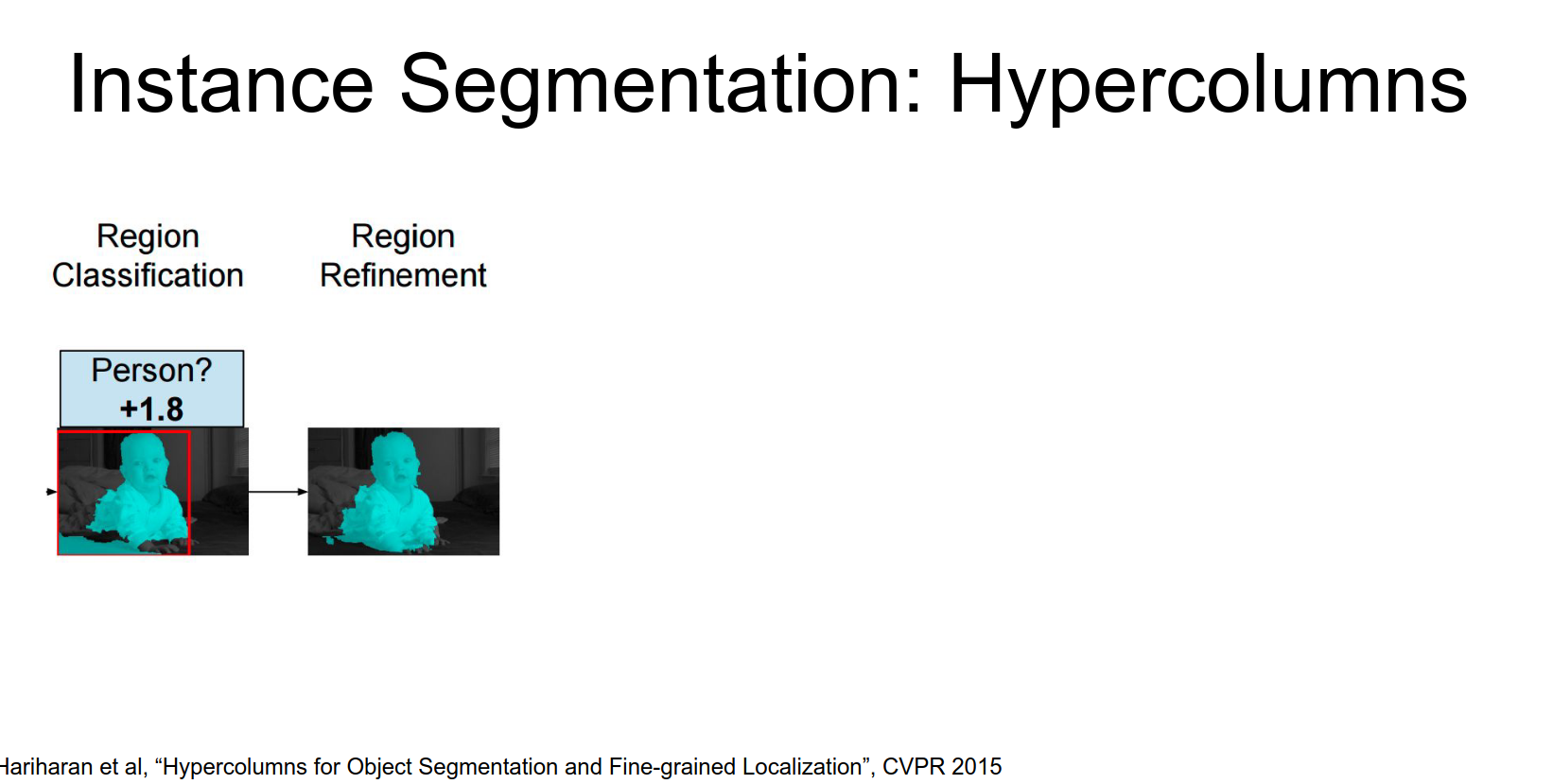
Here we're going to take out our image, crop out the box with corresponding to that segment and then pass it through an AlexNet and we're going to extract convolutional features from several different layers of that AlexNet.

For each of those feature maps will up sample them and combine them together and now will produce this proposed figure-ground segmentation.

So this this is actually kind of a funny output but it's really easy to predict the idea is that this output image we're just going to do a logistic classify or inside each independent pixel.

Given these features we just have a whole bunch of independent logistic classifiers that are predicting how much each pixel of this output is likely to be in the foreground or in the background

And they show that this type of multi scale refinement step actually cleans up the outputs of the previous system and gives quite nice results.

This actually is very similar to R-CNN but in the detection lecture we saw that R-CNN was just the start of the story, there's all these faster versions right?

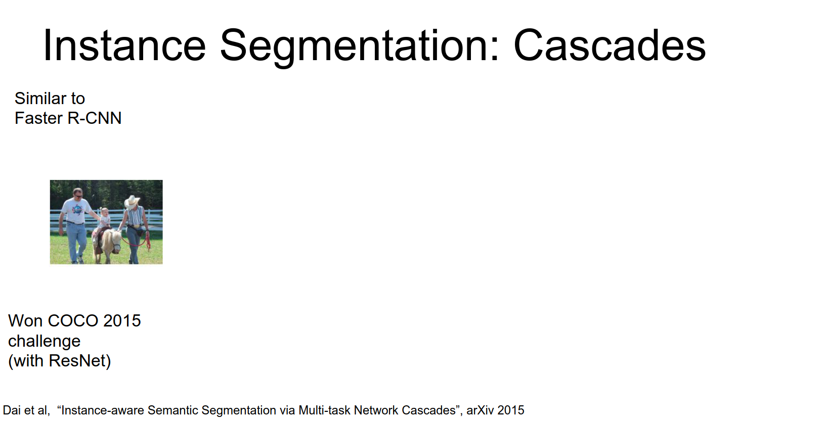
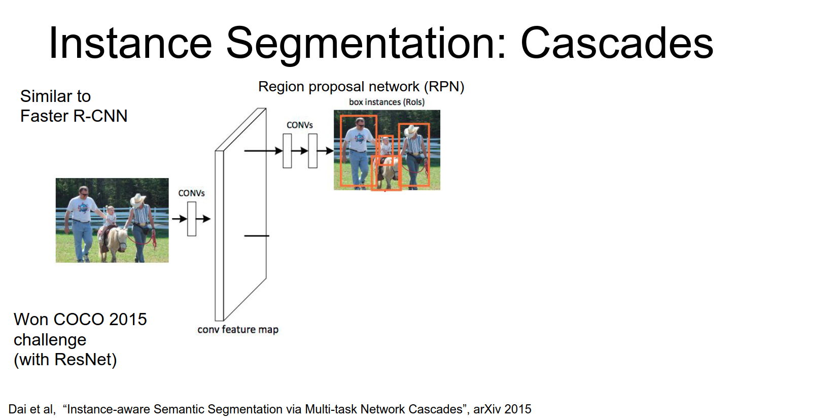
Mask R-CNN

A similar intuition from faster R-CNN has actually been applied to this instant segmentation problem as well.

Microsoft won the COCO instance segmentation challenge with a model similar to Faster R-CNN.

1. Input image goes through a CNN (ResNet).
2. RPN generates region proposals.
3. ROI Pooling extracts features for each proposal.

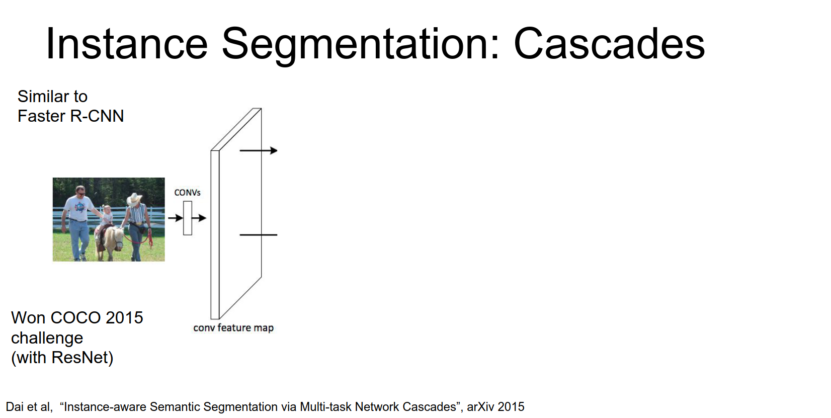
From this high resolution image we're actually going to propose our own region proposals.

In the previous method we relied on these external segment proposals, but here we're just going to learn our own region proposals just like Faster R-CNN.

Here we just stick a couple extra convolutional layers on top of our convolutional feature map and each one of those is going to predict several regions of interest in the image that using this idea of anchor boxes that we saw in the detection work.

1. For each region, predict a coarse segmentation mask and classify the object.
2. Mask out the background and classify again.

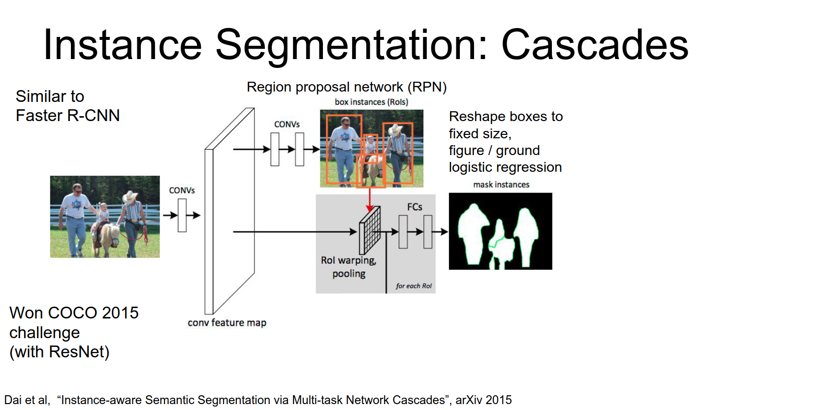
Now that we've predicted the foreground background for each of these, segments we're going to mask out the predicted background and only keep the pixels from the predicted foreground.

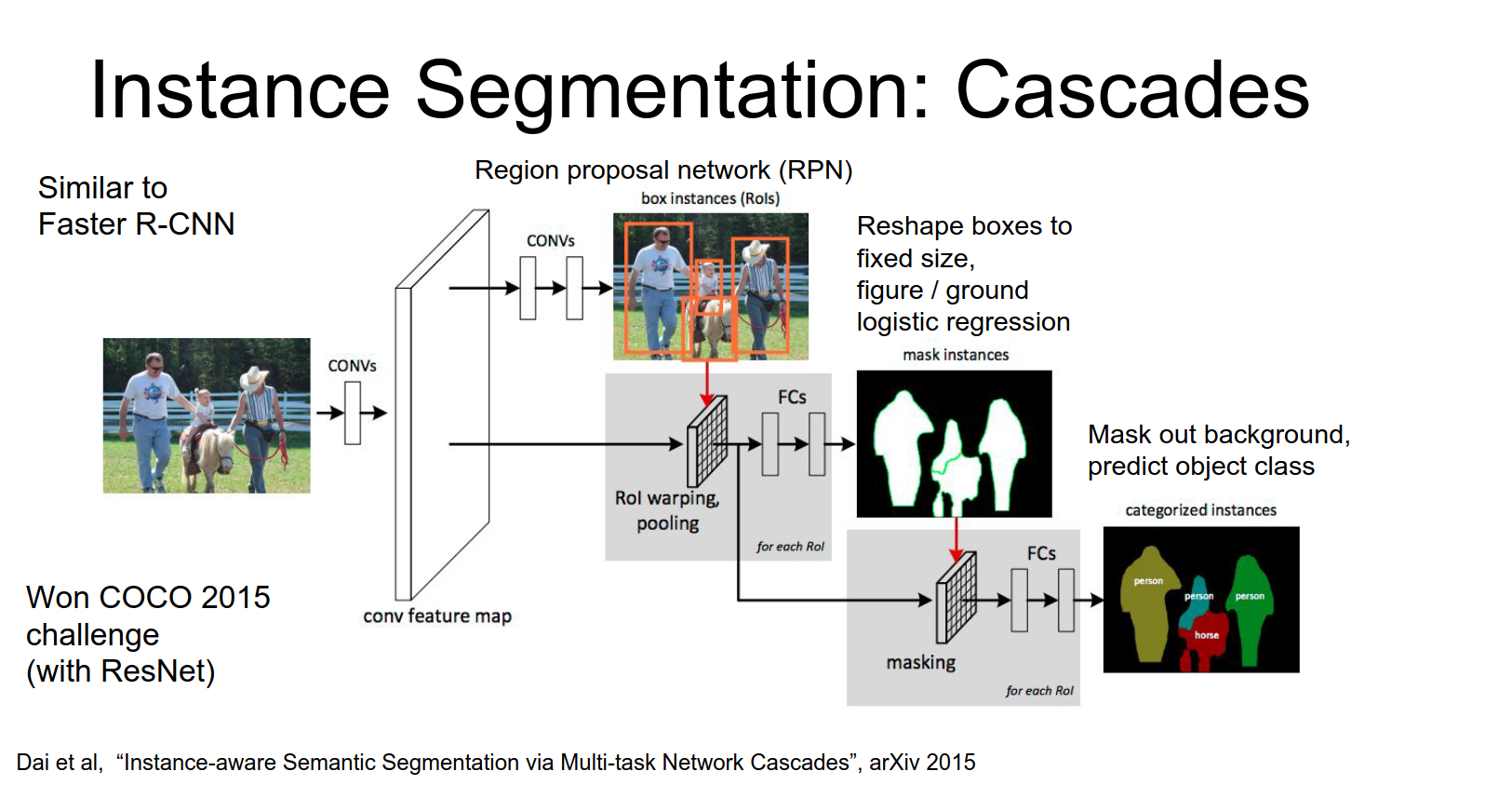
This is trained end-to-end.

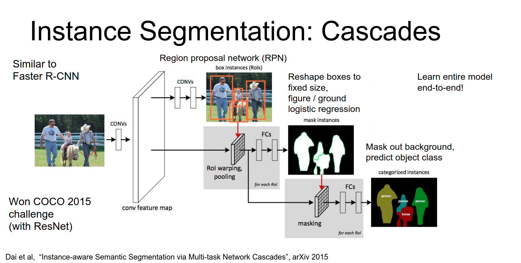
The results are very impressive, handling occlusion and multiple instances well.

Summary:

• Semantic Segmentation: Often uses Fully Convolutional Networks with learnable upsampling.
• Instance Segmentation: Often uses detection-based pipelines (like R-CNN variants) with segmentation heads.

Attention

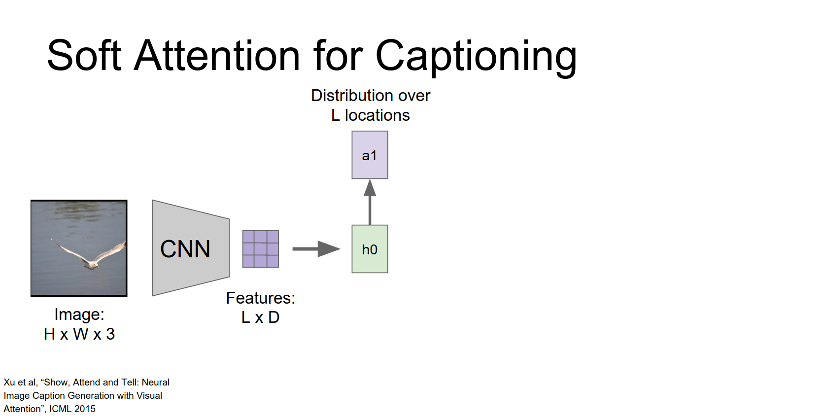
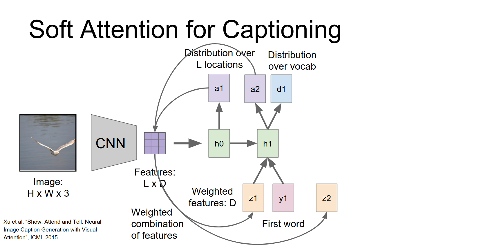
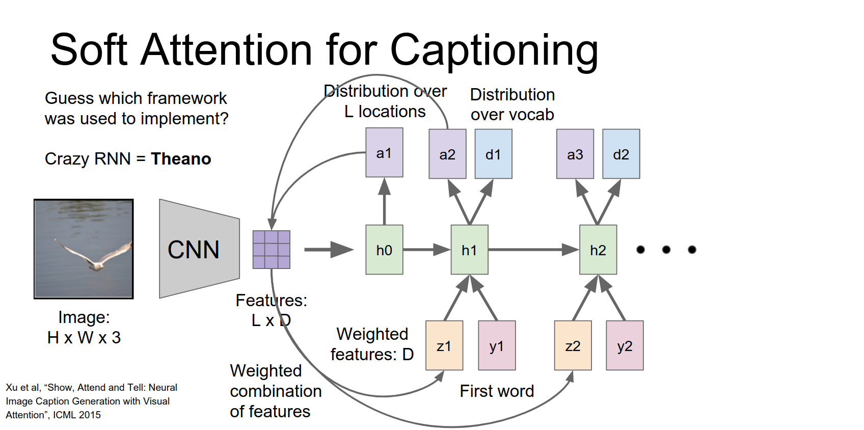
Attention has been a very popular topic recently. We'll look at it in the context of Image Captioning.

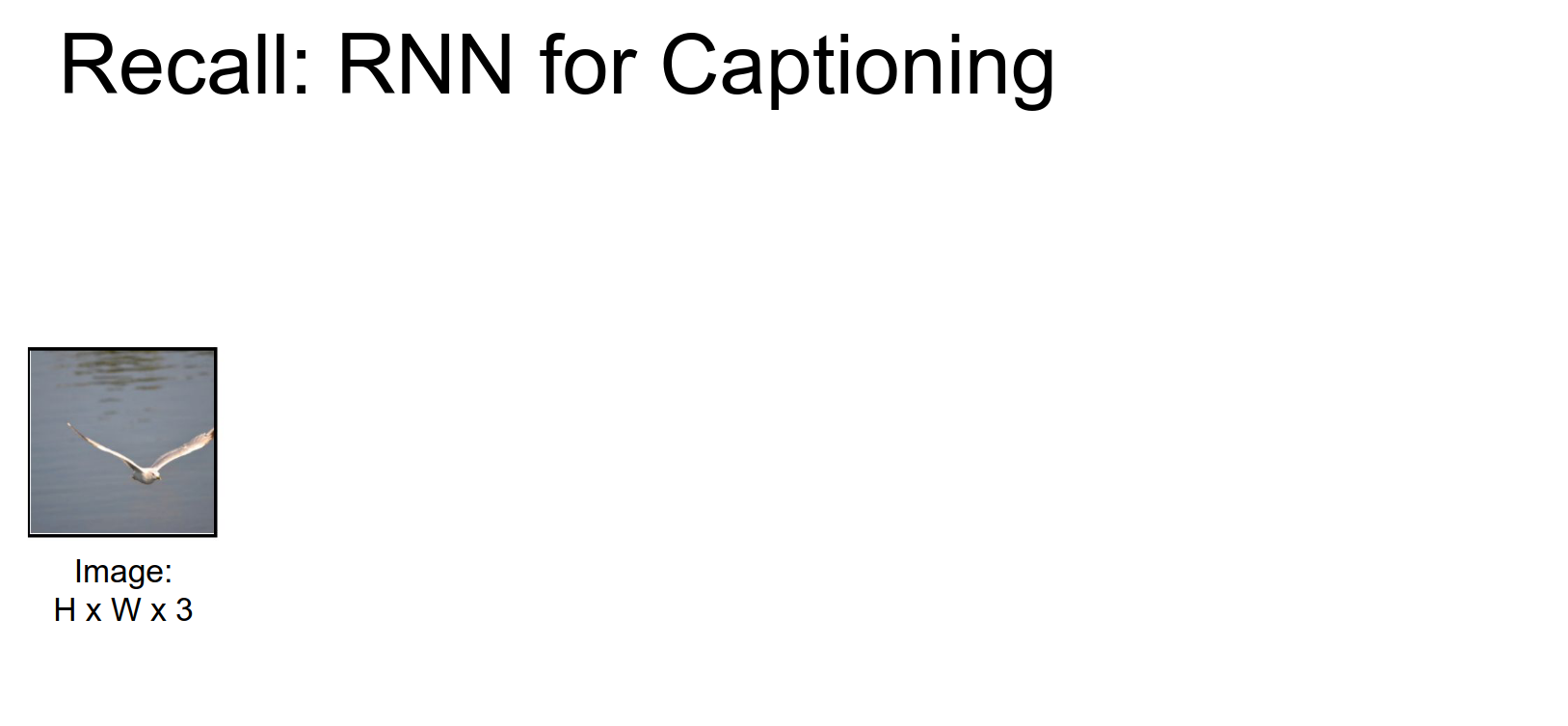
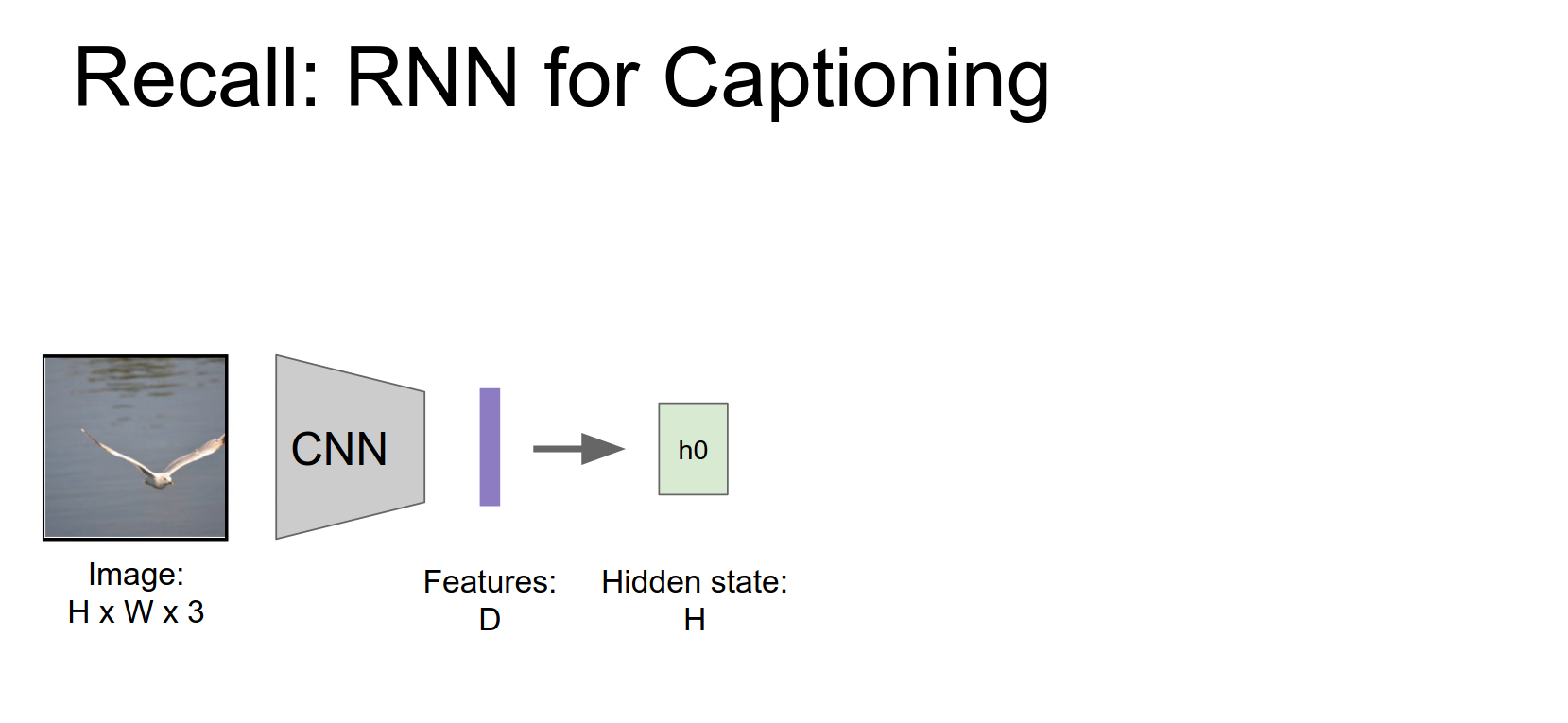
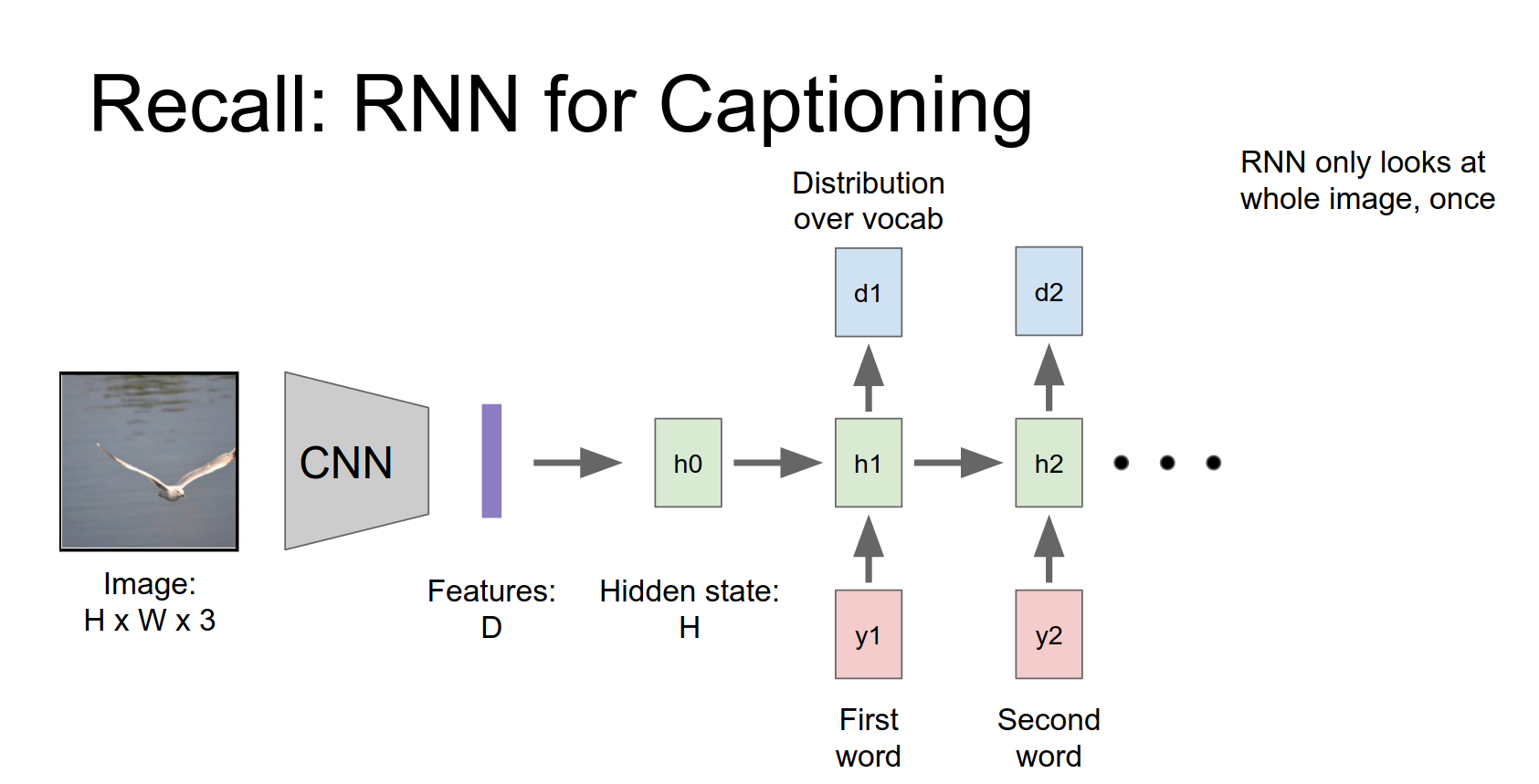
Recap of standard Image Captioning:

1. Input image -> CNN -> Features.
2. Initialize RNN hidden state with features.
3. RNN generates words one by one.

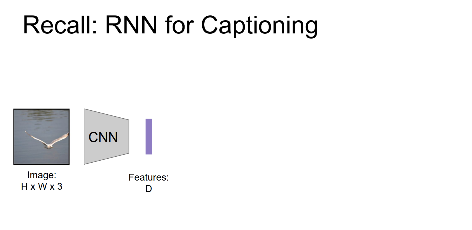
Those features will be used maybe to initialize the first hidden state of our RNN.

Then our start token or our first word together with that hidden state we're going to produce this distribution over words in our vocabulary.

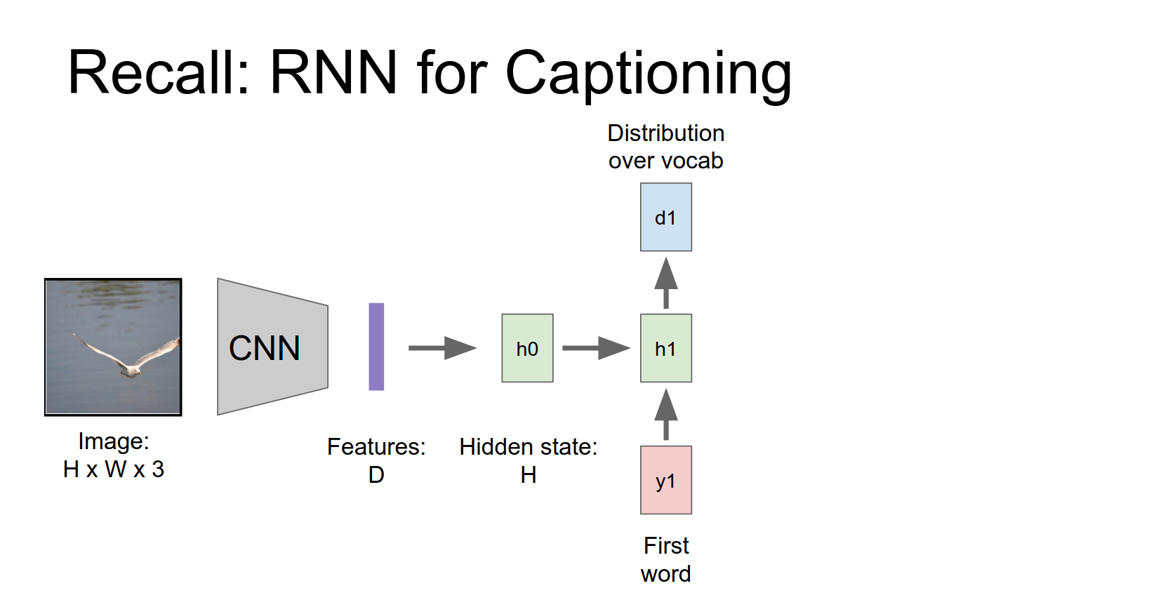
Then to generate a word we'll just sample from that distribution and we'll repeat this process over time to generate captions.

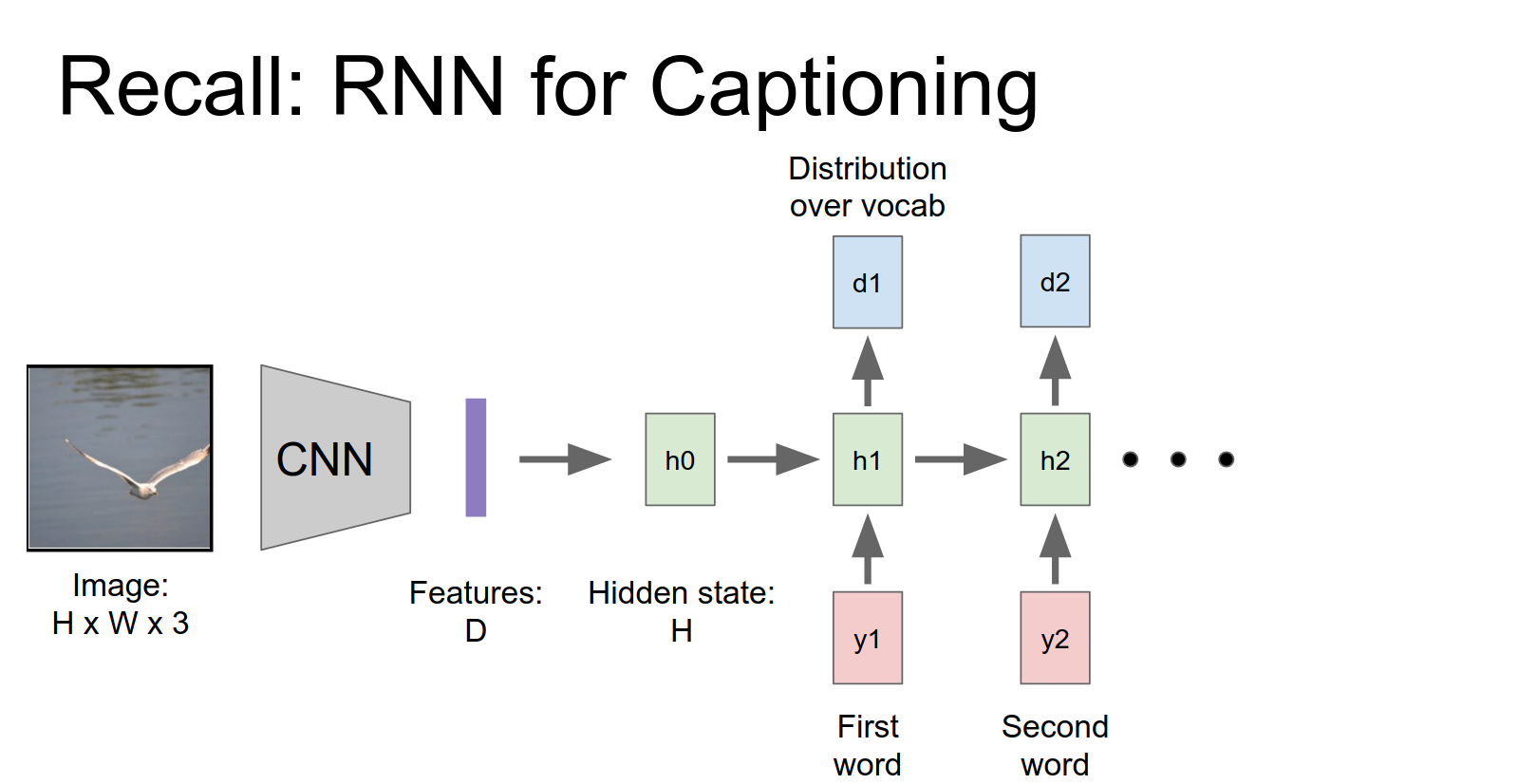
The problem is that the network looks at the entire image once and then has to generate the whole caption. It might be better if it could look at the image multiple times and focus on different parts as it generates words.

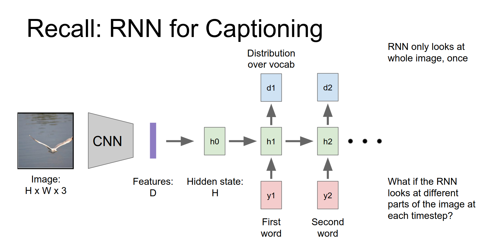
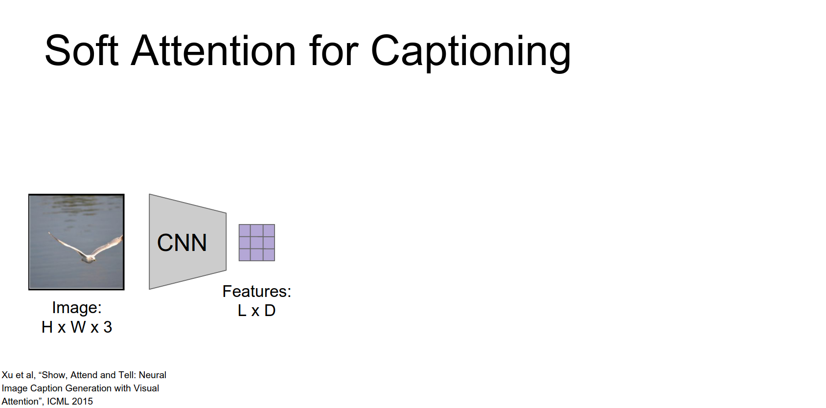
Show, Attend and Tell

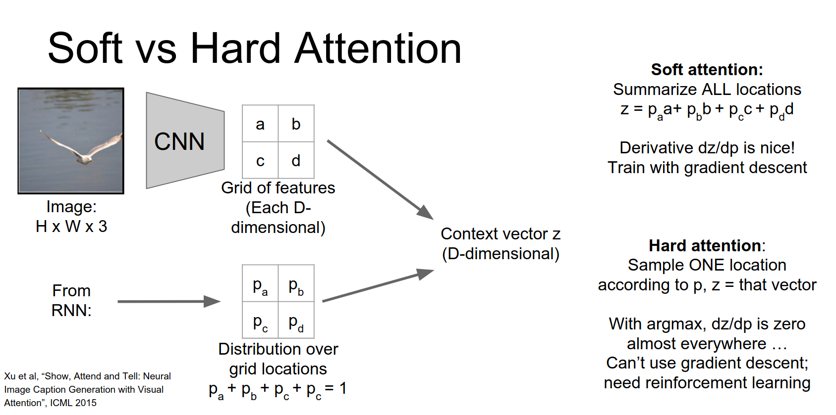
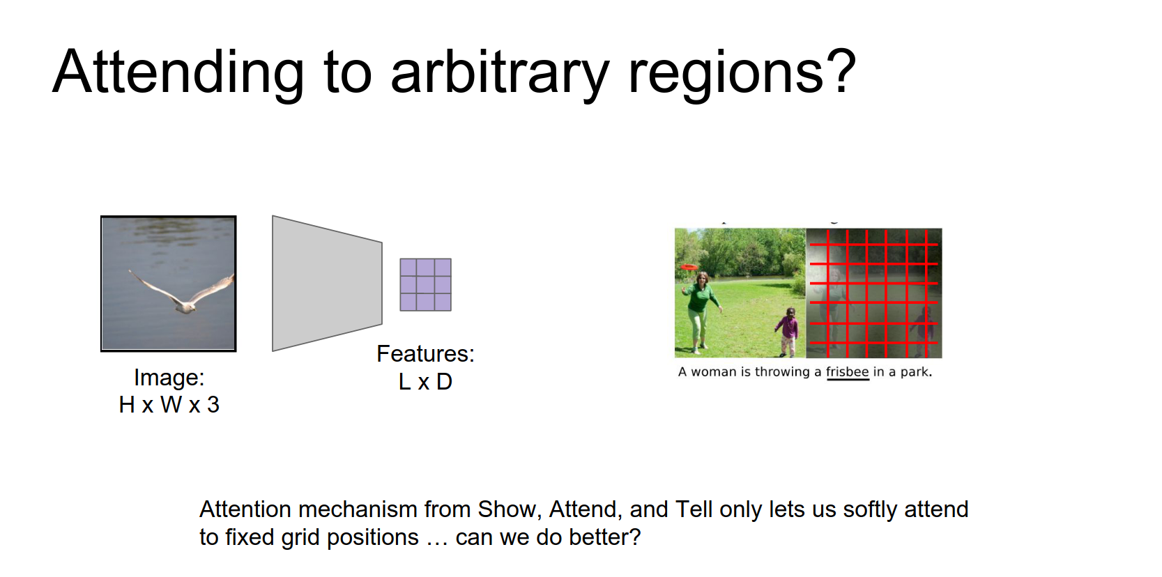
This paper introduced attention for captioning. Instead of using the final fully connected layer features, they use features from an earlier convolutional layer (e.g., \(14 \times 14 \times 512\)). This gives a grid of features corresponding to different spatial locations.

At each time step, the RNN produces a distribution over words AND a distribution over locations in the feature grid.

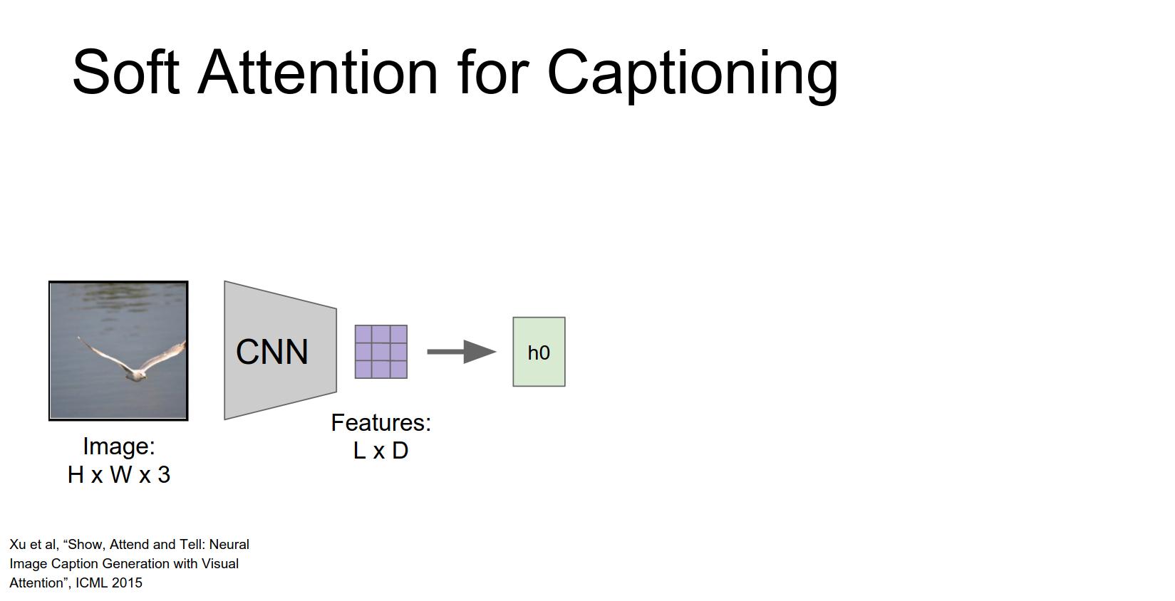
We're going to use our hidden state to compute not a distribution over words but instead a distribution over these different positions in our convolutional feature map.

We just end up with this l dimensional vector giving us a probability distribution over these different locations in our input.

This distribution is used to compute a weighted sum of the feature vectors (the context vector \(z\)).

This vector summarizes the image by focusing on specific parts.

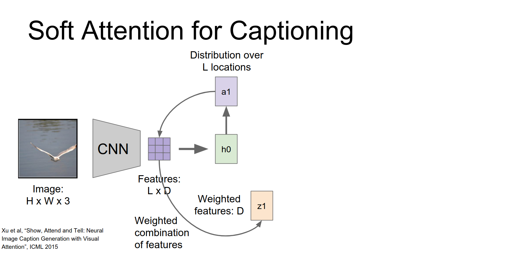
The RNN receives three inputs: previous hidden state, context vector \(z\), and the previous word.

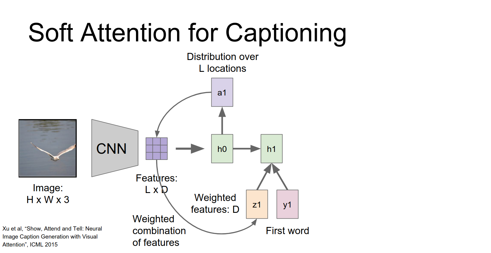
It produces a new hidden state, a new word distribution, and a new location distribution.

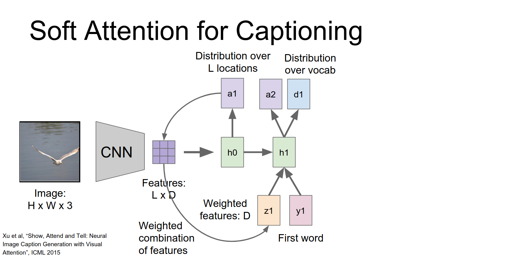
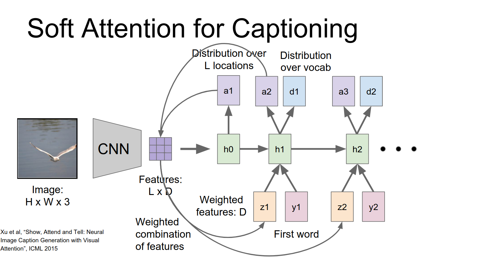
And now this process repeats.

So given this new probability distribution we go back to the input feature grid and compute new summarization vector for the image.

Take the take that vector together with the next word in the sentence to compute the new hidden state.

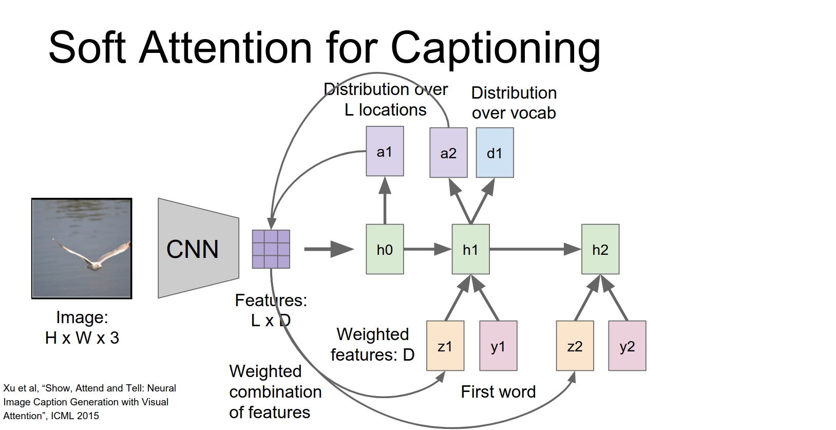
This repeats over time to generate our captions.

Q: Where does this feature grid come from?

A: The answer is when you're when you're doing an AlexNet for example you have Conv 1 Conv 2 Conv 3 Conv 4 Conv 5 and by the time you get to Conv 5 the shape of that tensor is now something like \(7x7x512\).

So that corresponds to a seven by seven spatial grid over the input and in each a grid position that's a 512 dimensional feature vector. Those are just pulled out of one of the convolutional layers in the network.

What framework you wanted to use to implement this?

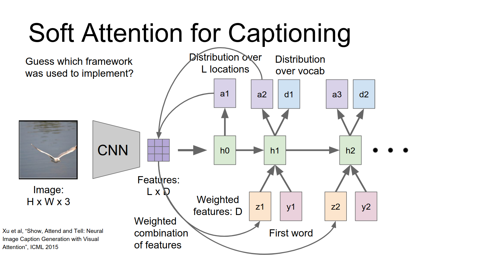
We talked about maybe how RNN's would be a good choice for Theano or TensorFlow and I think this qualifies as a crazy RNN.

There are two ways to compute the context vector: Soft Attention and Hard Attention.

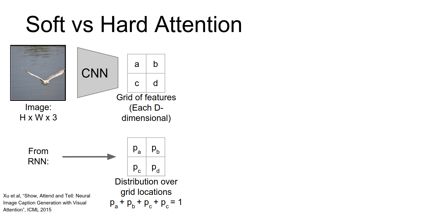
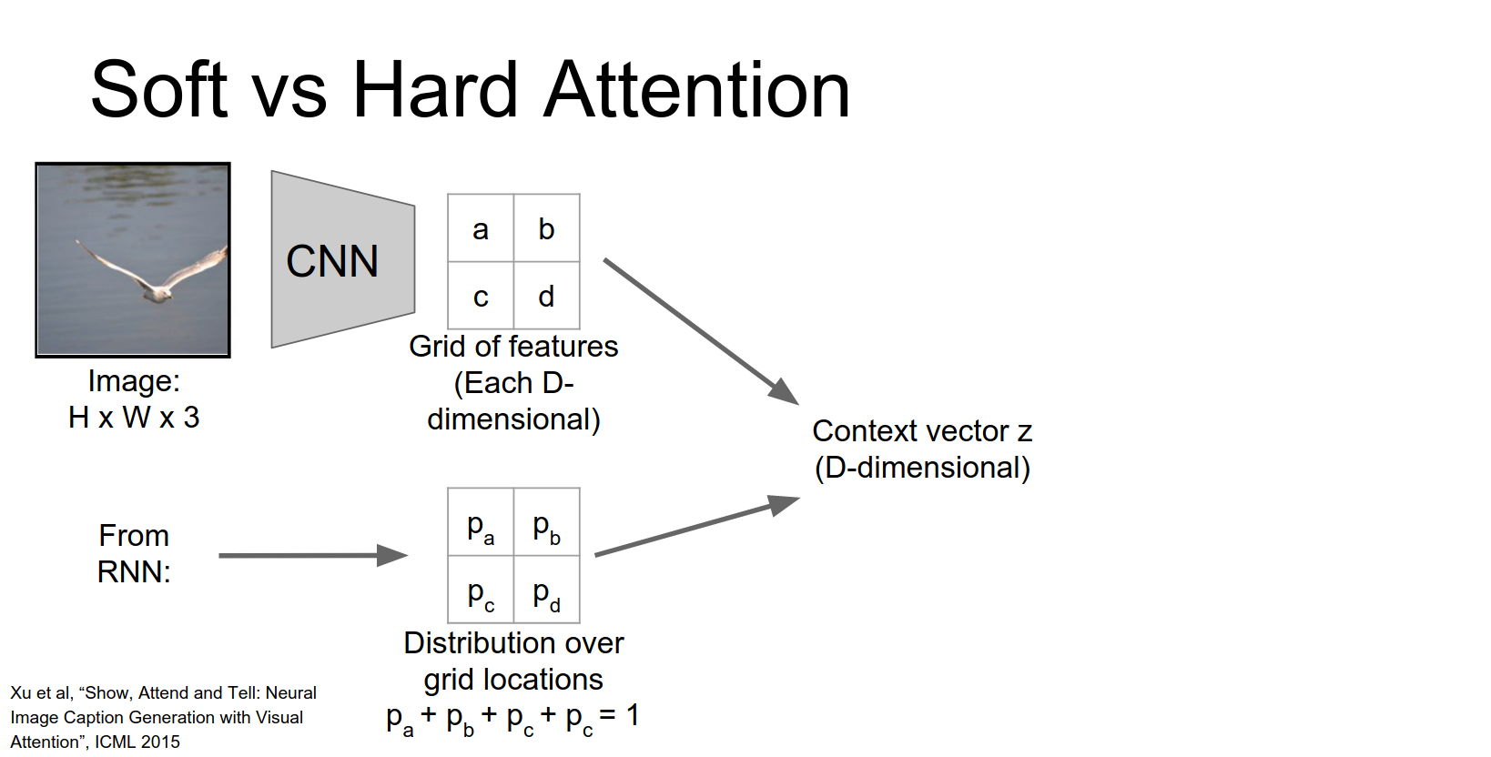
Soft Attention

In soft attention, the context vector \(z\) is a weighted sum of the grid features, weighted by the predicted probability distribution.

This is fully differentiable and can be trained with standard backpropagation.

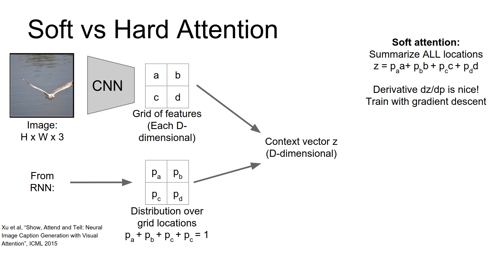
Hard Attention

Instead of having this weighted sum we might want to select just a single element of that grid to attend to.

One simple thing to do is just to pick the element of the grid with the highest probability and just pull out the feature vector corresponding to that argmax position.

The problem is now if you think about in this argmax case, if you think about this derivative the derivative of Z with respect to our distribution P, it turns out that this is not very friendly for back propagation anymore.

So imagine in an argmax case, suppose that a that \(P_{a}\) were actually the largest element in our input. And now what happens if we change \(P_{a}\) just a little bit?

So if \(P_{a}\) is the argmax and then we just jiggle the probability distribution just a little bit then \(P_{a}\) will still be the argmax.

So we'll still select the same vector from the input.

Which means that actually the derivative of this vector Z with respect to our predicted probabilities is going to be zero almost everywhere.

So that's very bad, we can't really use back propagation anymore to train this thing.

In hard attention, we sample a single location from the distribution (or take the argmax).

This is not differentiable (gradients are zero almost everywhere). To train this, you need Reinforcement Learning.

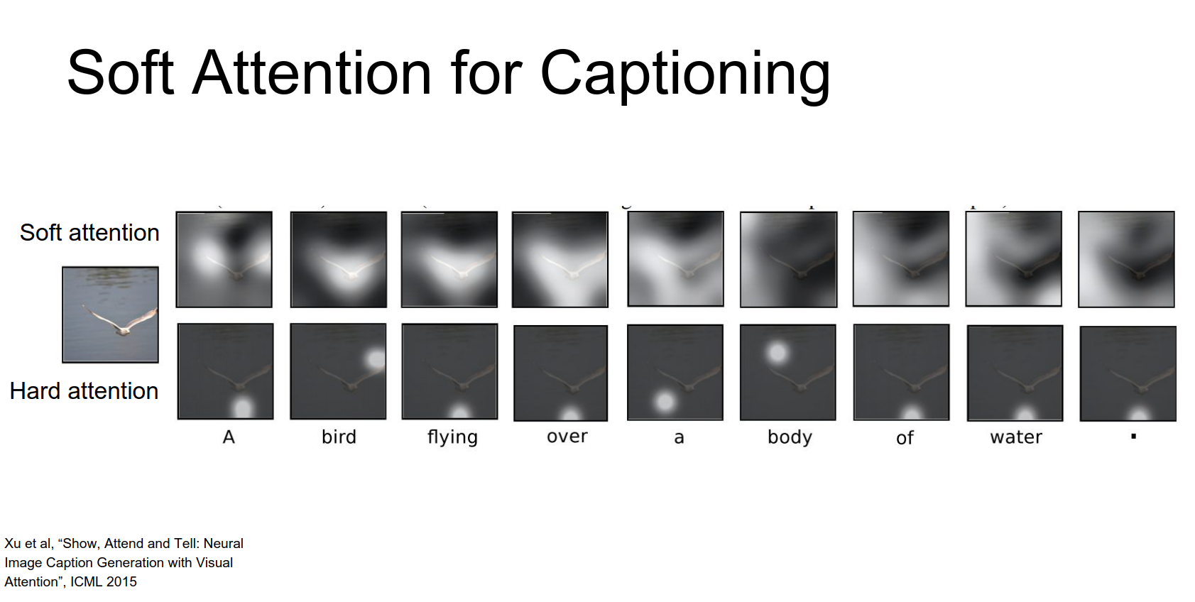
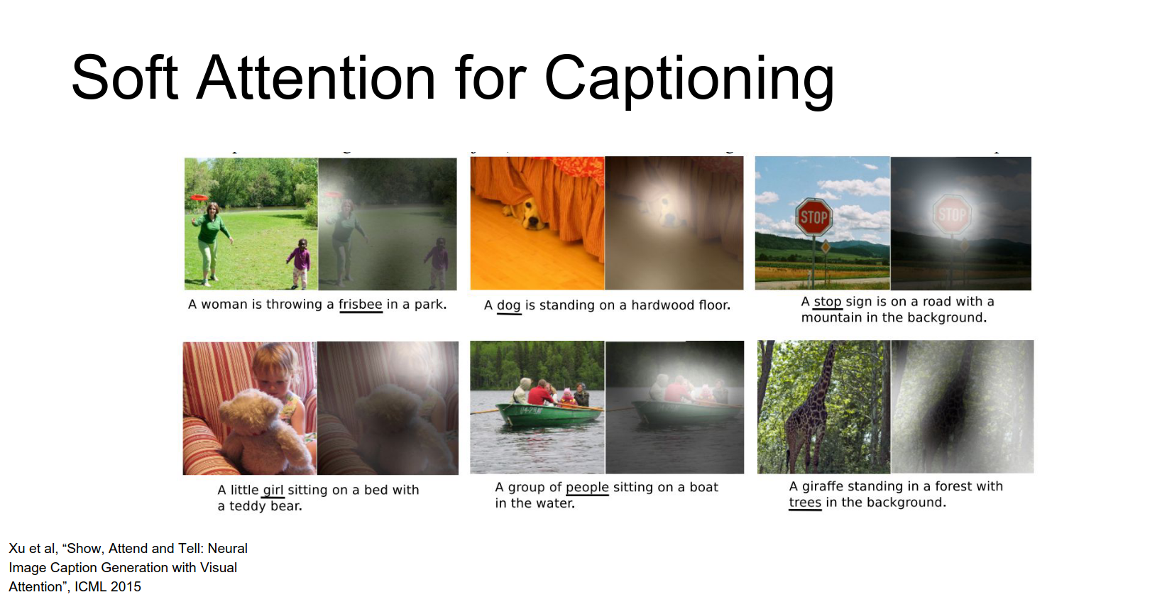
Results: The model learns to focus on relevant parts of the image.

• "Bird": focuses on the bird.
• "Water": focuses on the background.
• "Frisbee": focuses on the frisbee.

For this input image that shows a bird, they both their heart attention model and they're soft attention model in this case both produce the caption a bird flying over a body of water period.

And for these two models they've visualized what that probability distribution looks like for these two different models.

The top shows the soft attention so you can see that it's sort of diffused since it's averaging probabilities from every location and image, and in the bottom it's just showing the one single element that it pulled out.

These actually have quite nice semantic interpretable meanings.

Q: When would you prefer hard versus soft attention ? 🏂

When you have a very large input it might be computationally expensive to actually process that whole input on every time step.

And it might be more efficient computationally if we can just focus on one part of the input at each time step, and only process a small subset per time step.

So with soft attention because we're doing this sort of averaging over all positions we don't any computational savings we're still processing the whole input on every time step

but with hard attention we actually do get a computational savings since we're explicitly picking out some small subset of the input

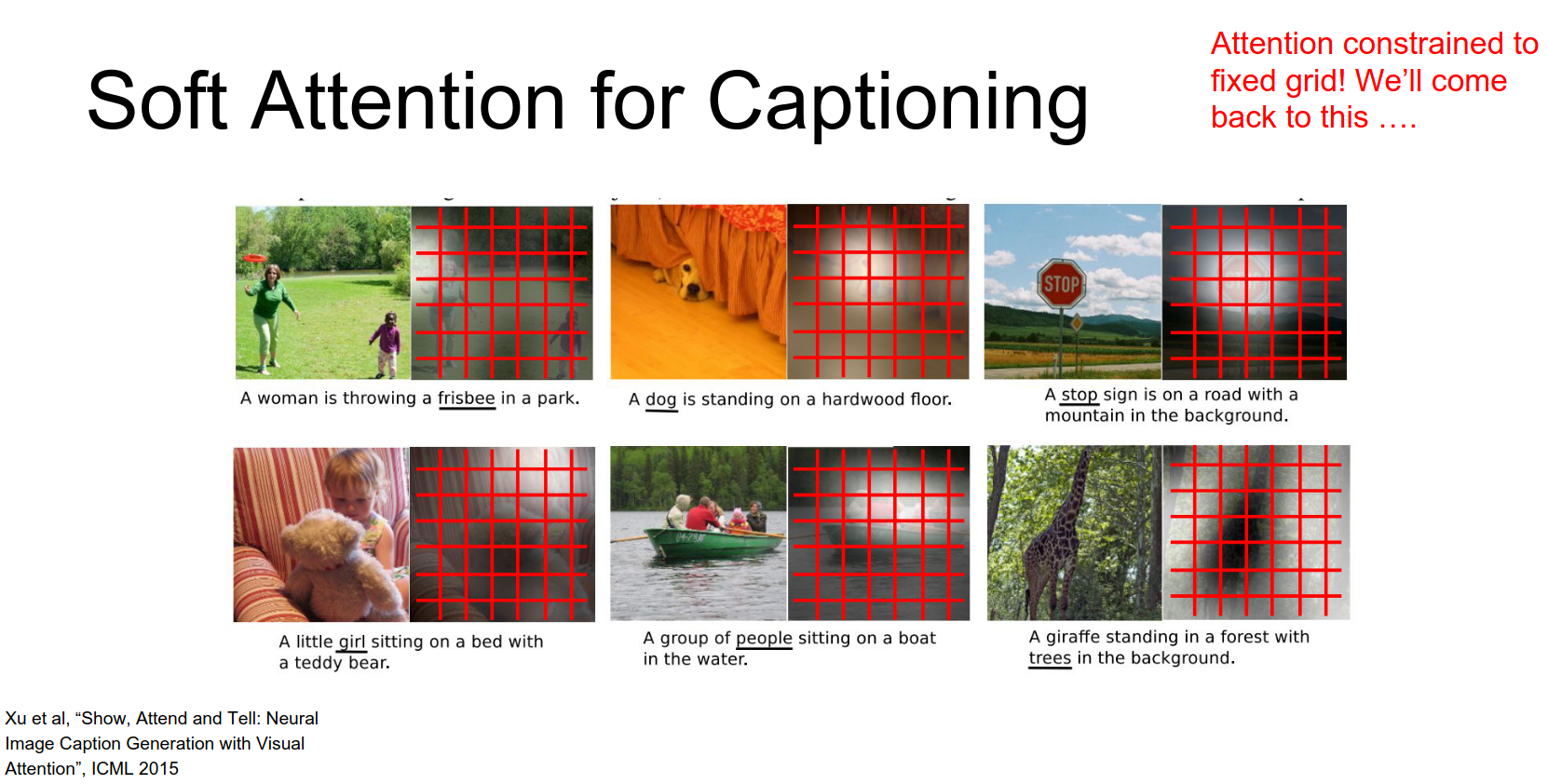
Constraint: Soft attention is constrained to the fixed grid of the convolutional feature map. It cannot attend to arbitrary regions.

Attention in Other Domains

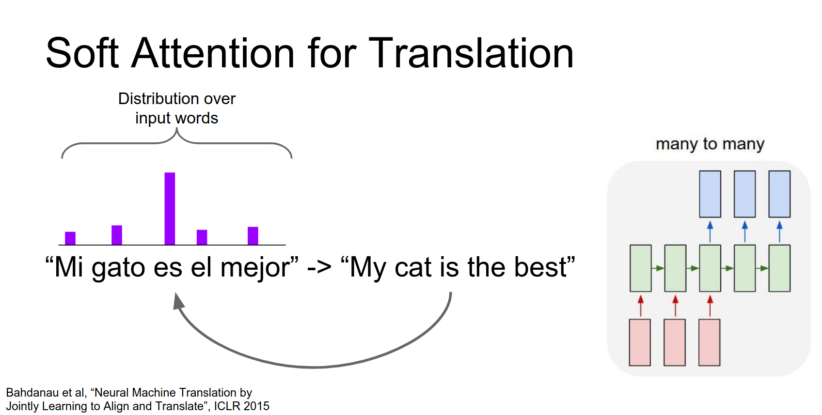
Attention originated in Machine Translation (Bahdanau et al., 2014).

• Attend to words in the input sentence while generating the output sentence.
• Uses content-based addressing (dot products) to handle variable-length sequences.

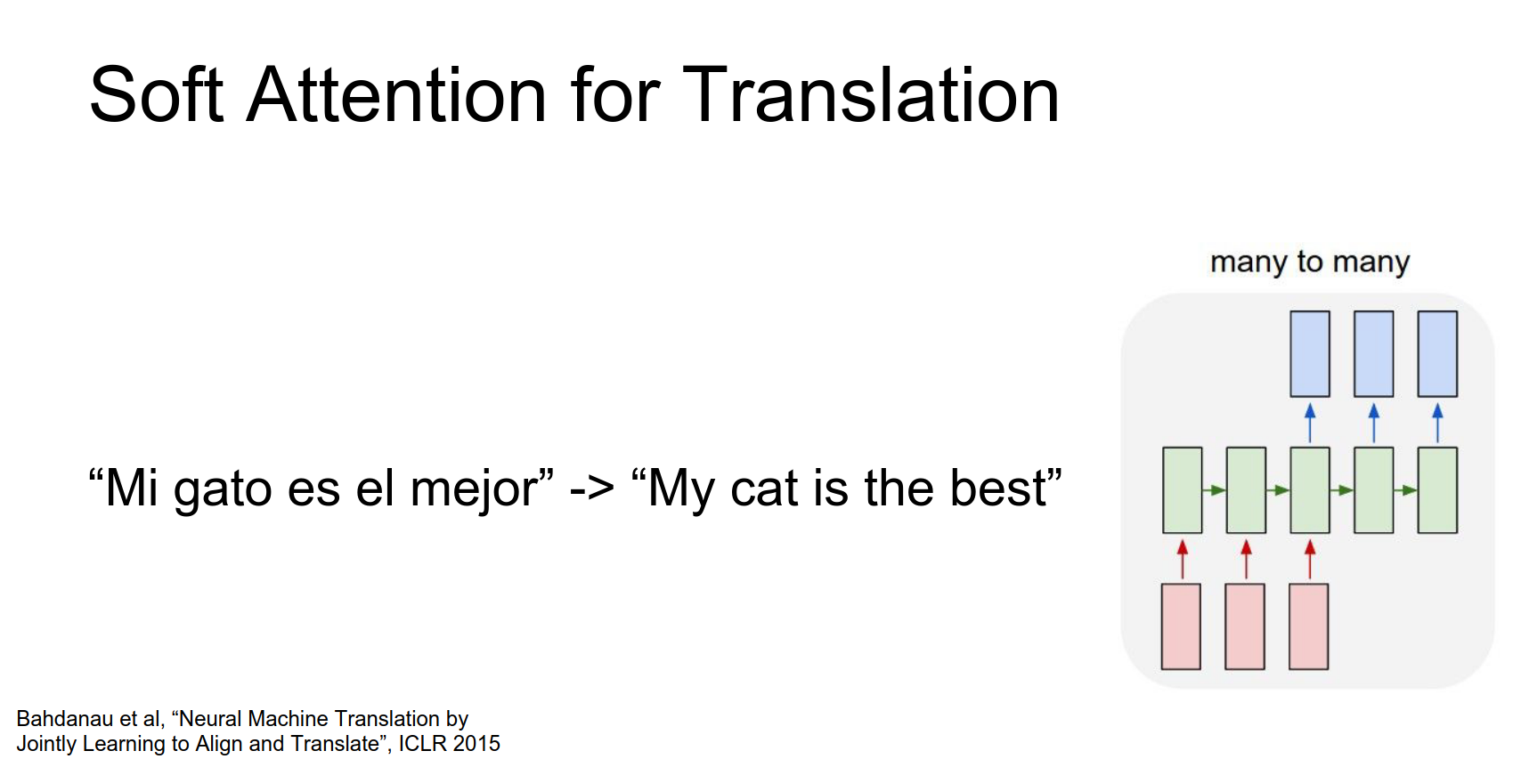
When we generate this first word my we want to compute a probability distribution not over regions in an image but instead over words in the input sentence.

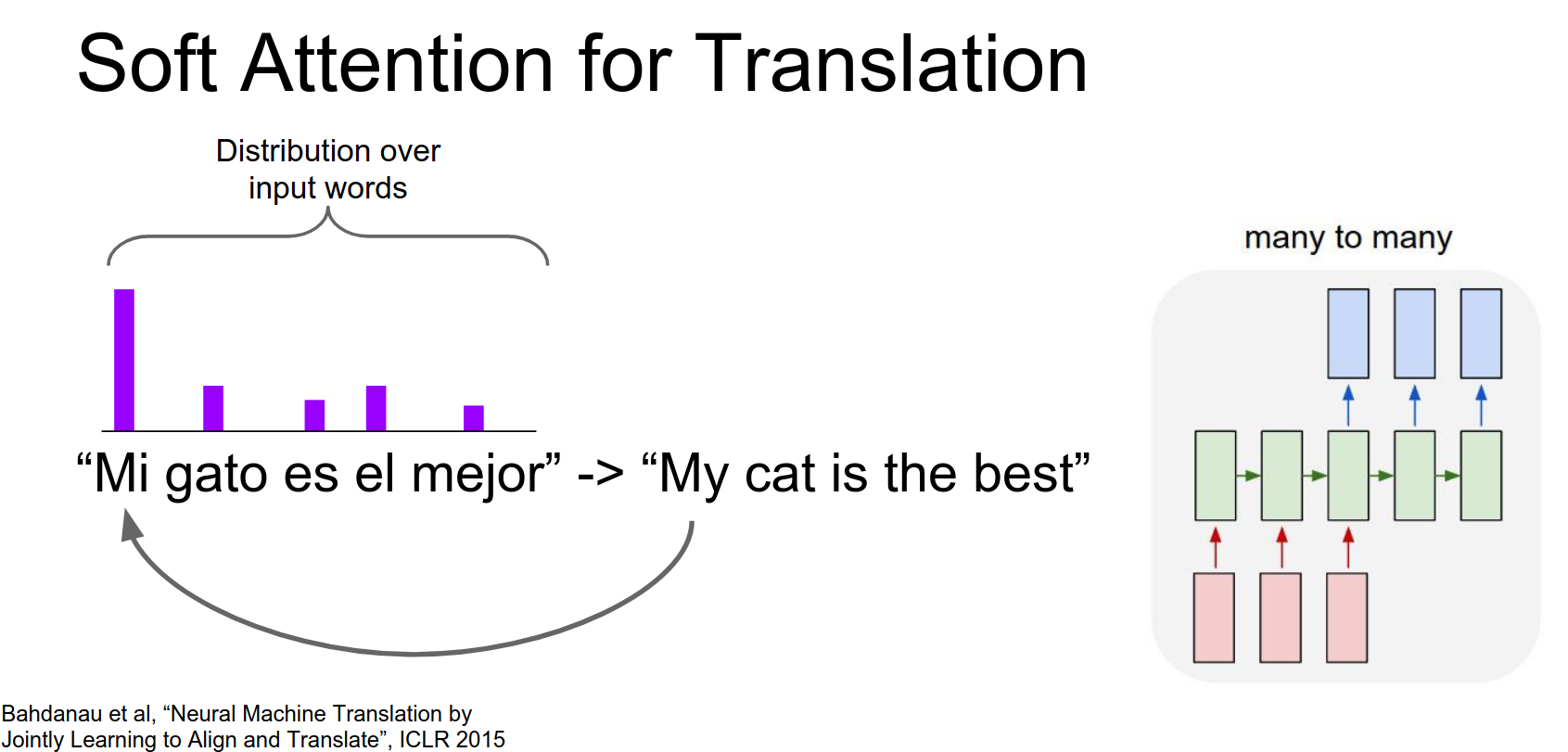
This process would repeat at every time step of the network.

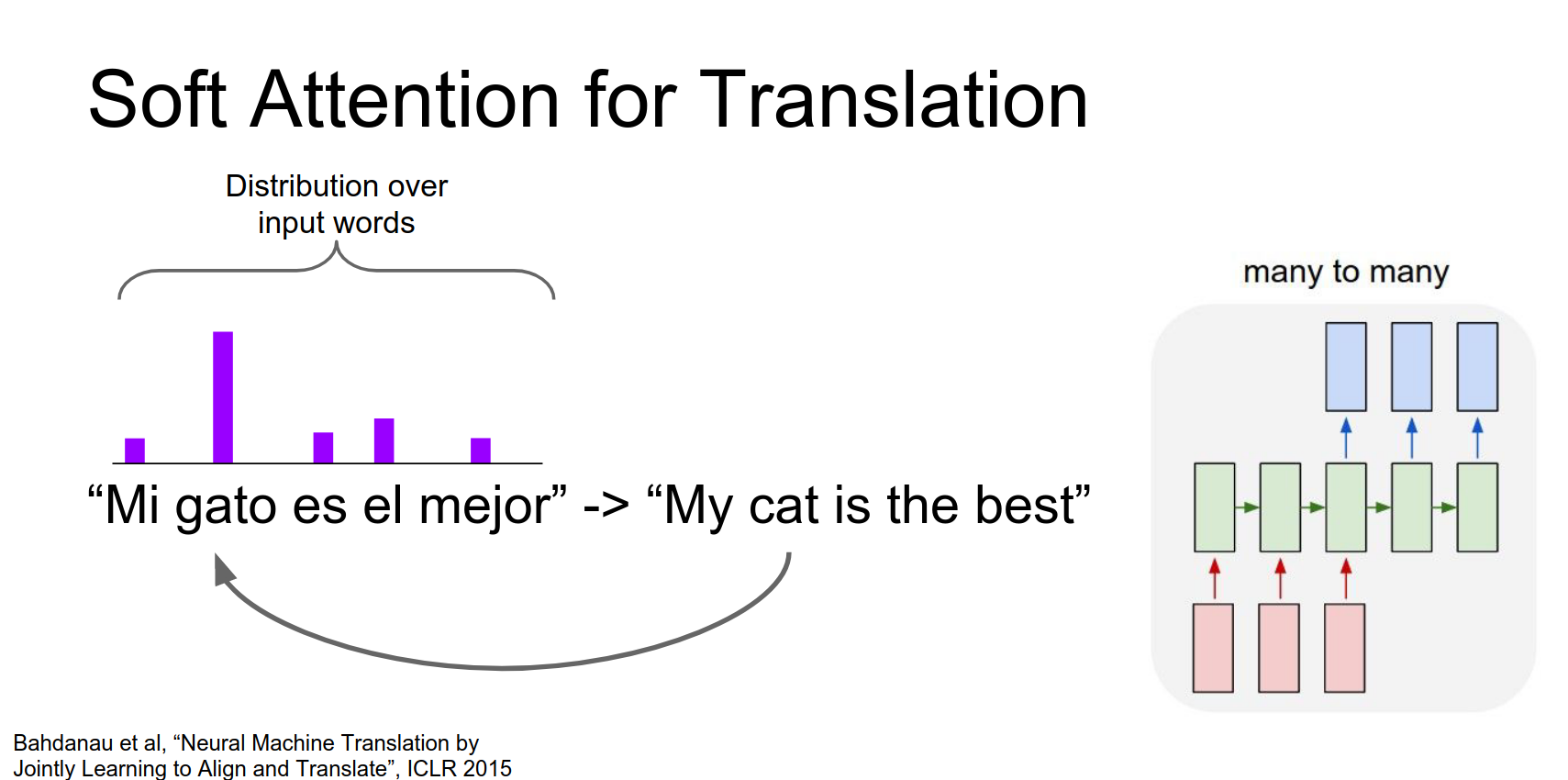
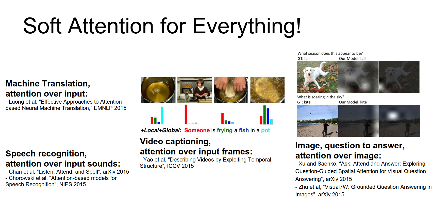
Soft attention is very easily applicable not only to image captioning but also to machine translation.

Other applications:

• Speech Recognition: "Listen, Attend and Spell".
• Video Captioning: Attend to frames.
• Visual Question Answering: "Ask, Attend and Answer".

Attending to Arbitrary Regions

Can we attend to arbitrary regions in a differentiable way?

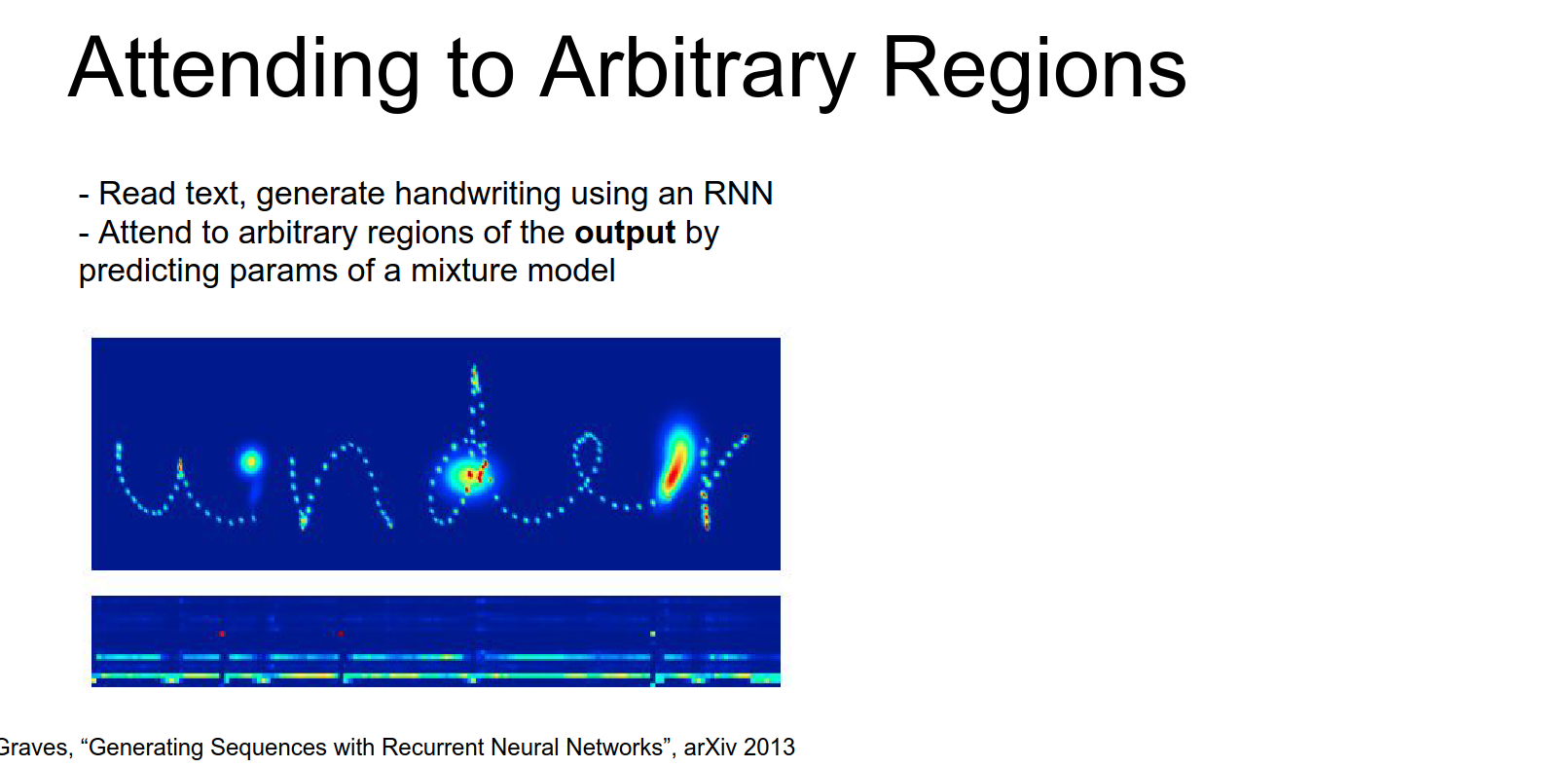
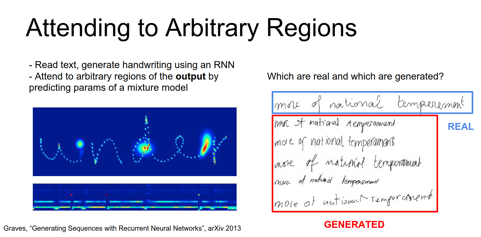
Handwriting Generation (Alex Graves, 2013): Used Gaussian mixture models to attend to continuous locations in the output sequence.

So here he wanted to read as input a natural language sentence and then generate as output actually an image that would be handwriting - writing out that that sentence in handwriting.

This actually has attention over this put image in kind of a cool way where now he's actually predicting the parameters of some Gaussian mixture model over the output image and then uses that to actually attend to arbitrary parts of the output image.

So on the right some of these are actually written by people and the rest of them were written by his network.

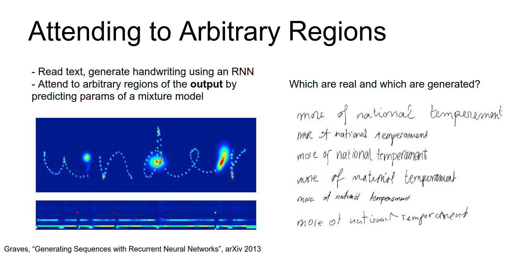
Top one is real and these bottom four are all generated by the network.

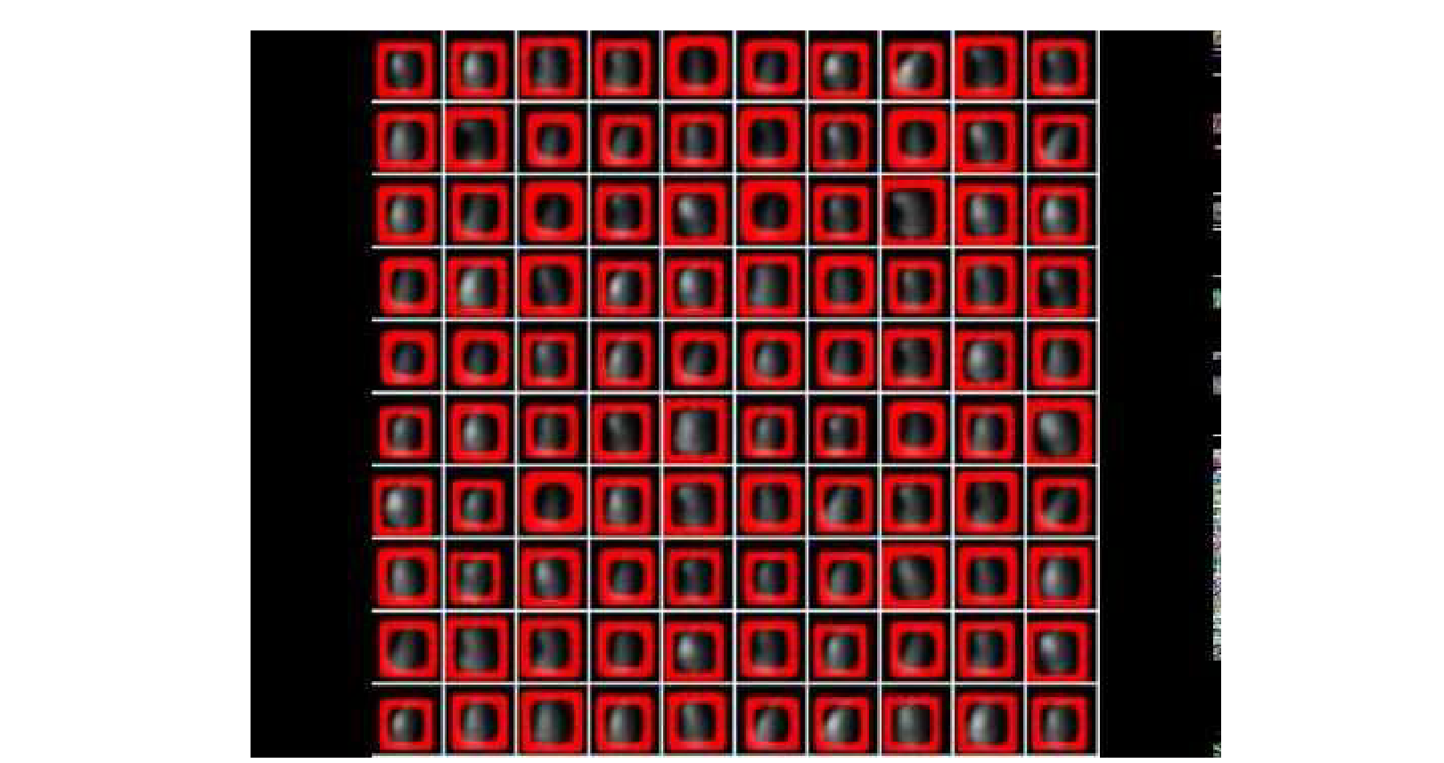
DRAW (Gregor et al., 2015): Used a similar mechanism for image generation and classification. It learns to attend to and "draw" the image step-by-step.

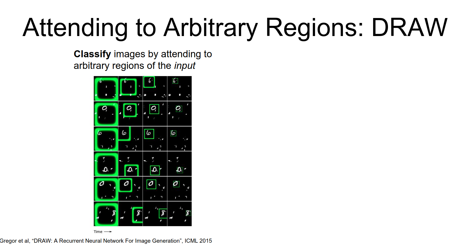
With Draw they also consider the idea of generating arbitrary output images with a similar sort of motivation as the handwriting generation. Where we're going to have arbitrary attention over the output image and just generate this output on bit by bit.

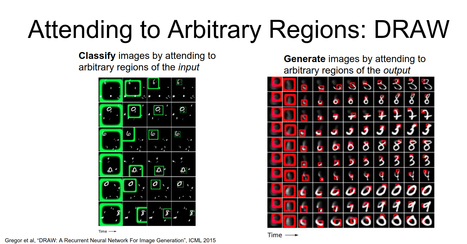
As you could see like the region it was attending to it was actually growing and shrinking over time and sort of moving continuously over the image and it was definitely not constrained to a fixed grid like we saw it with Show Attend and Tell.

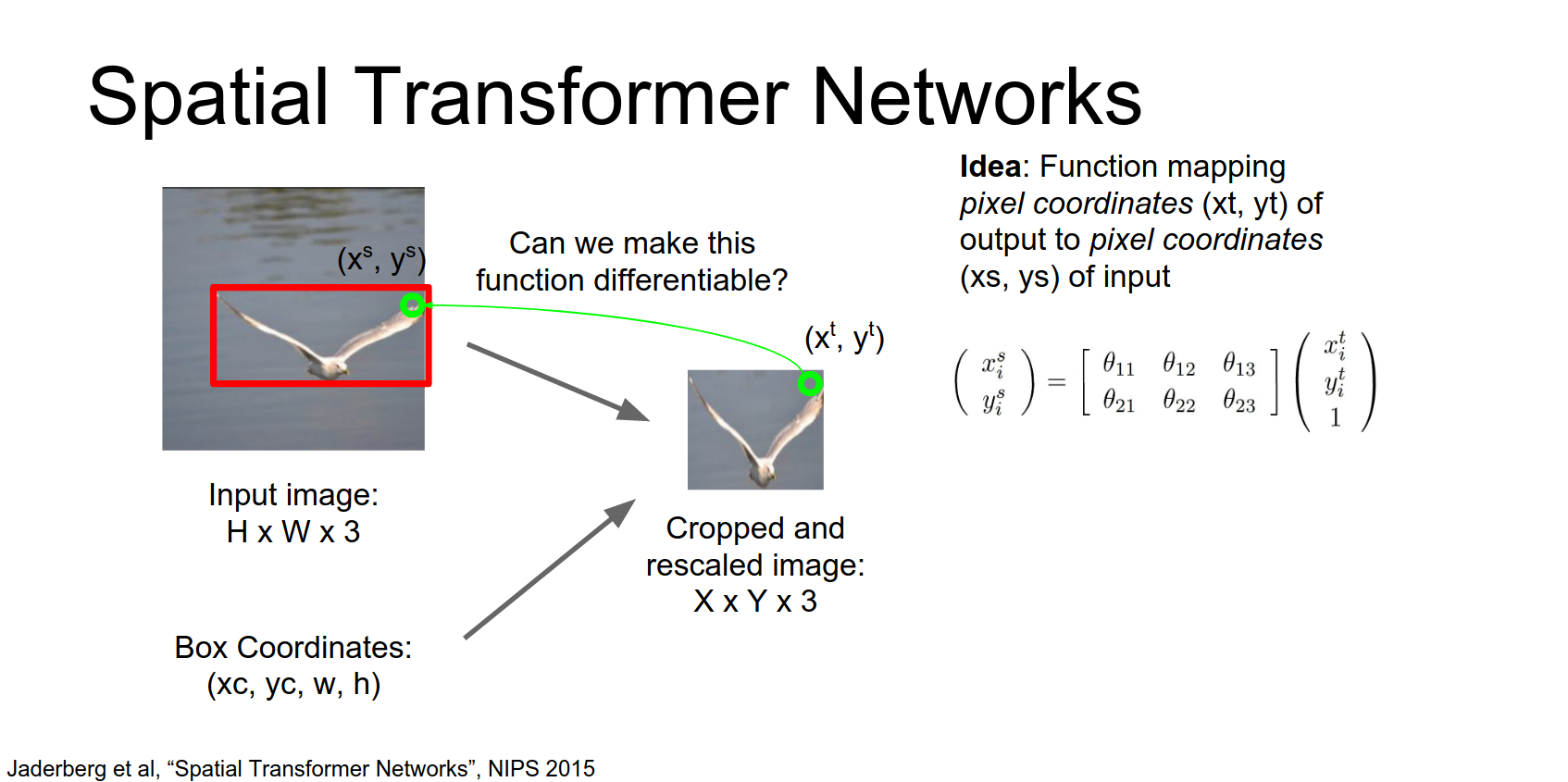
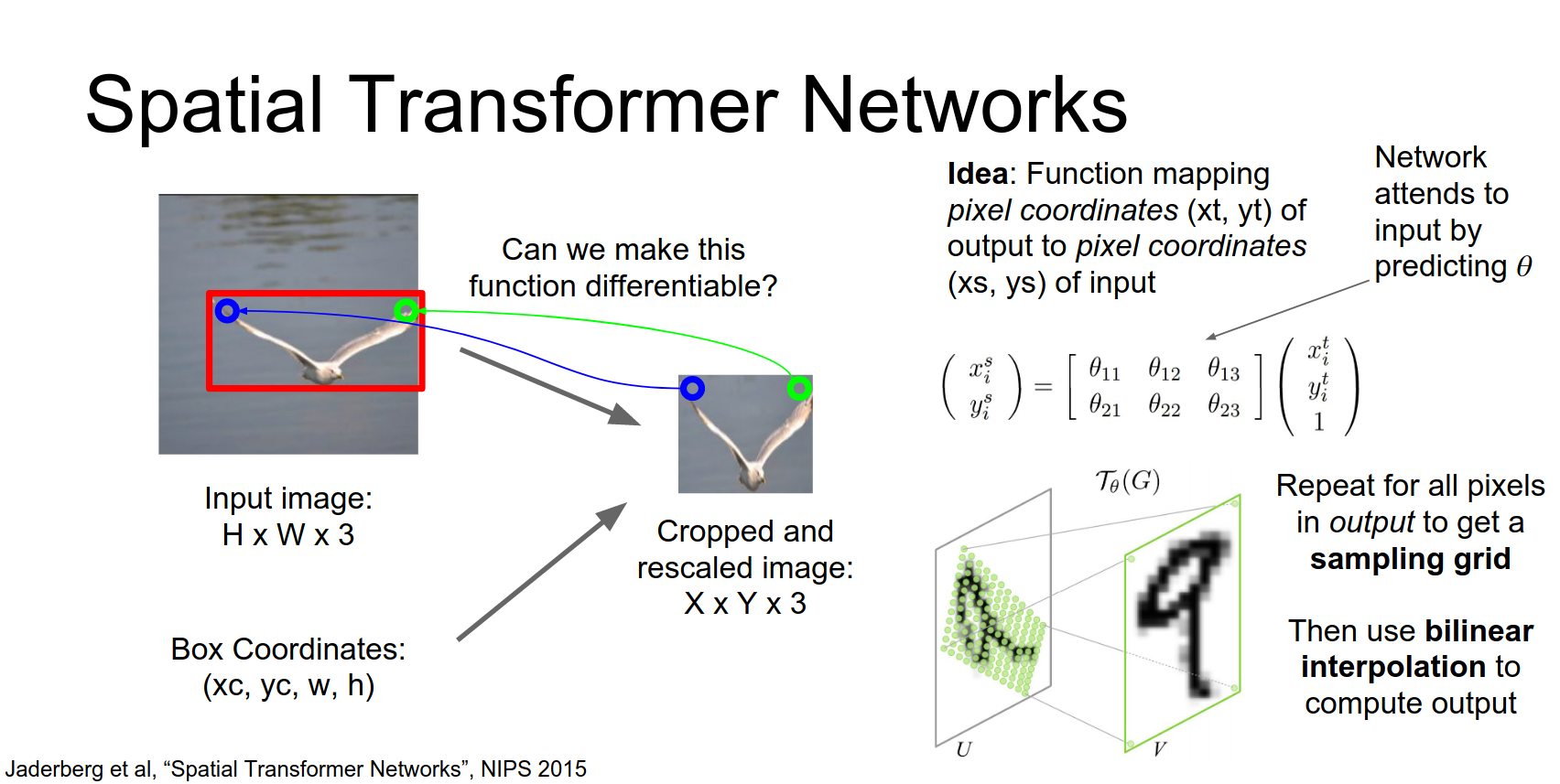
Spatial Transformer Networks

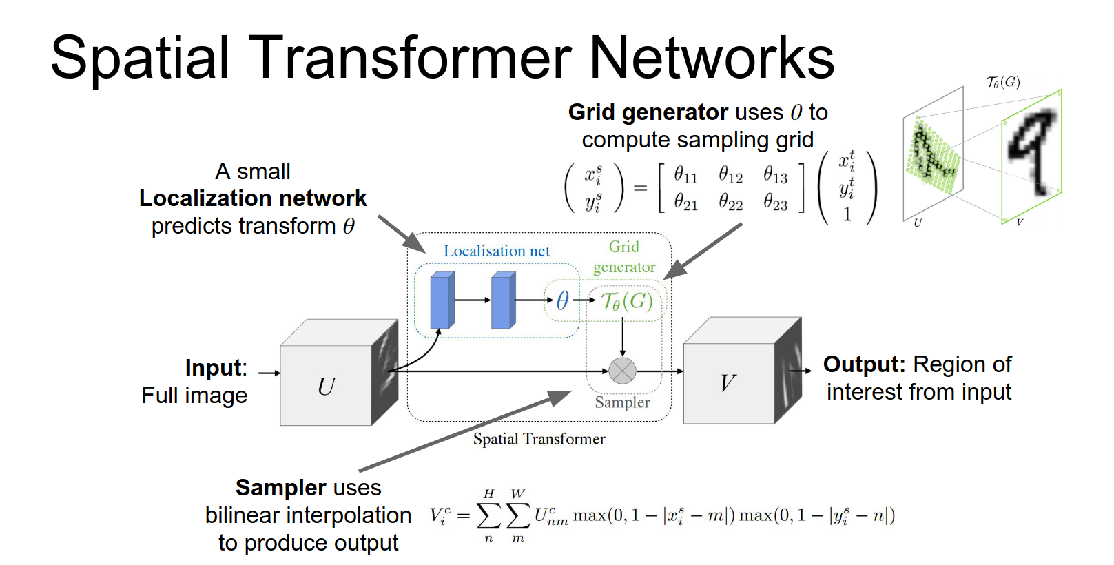
A cleaner way to do arbitrary attention is Spatial Transformer Networks (Jaderberg et al., 2015).

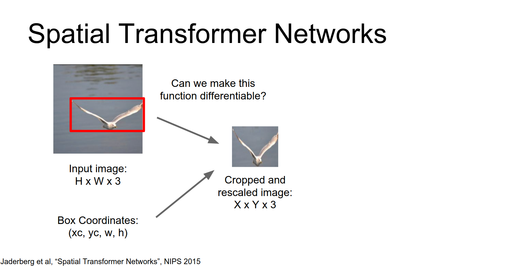
Idea: We want to predict continuous attention parameters (e.g., zoom, rotation, translation) and extract a transformed box from the input.

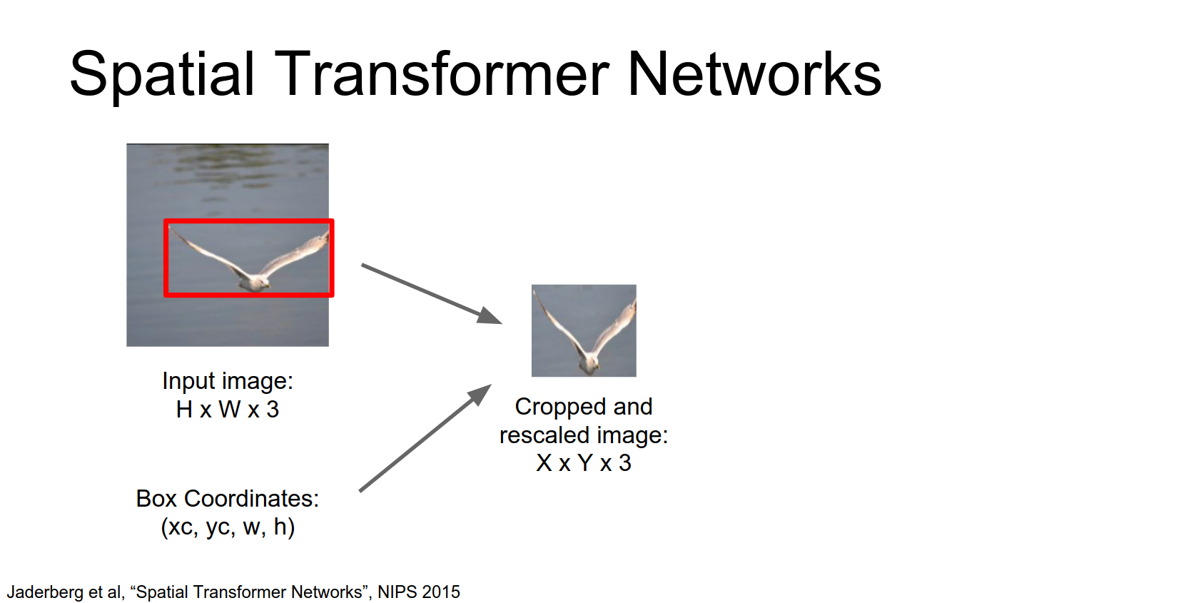
How to make this differentiable?

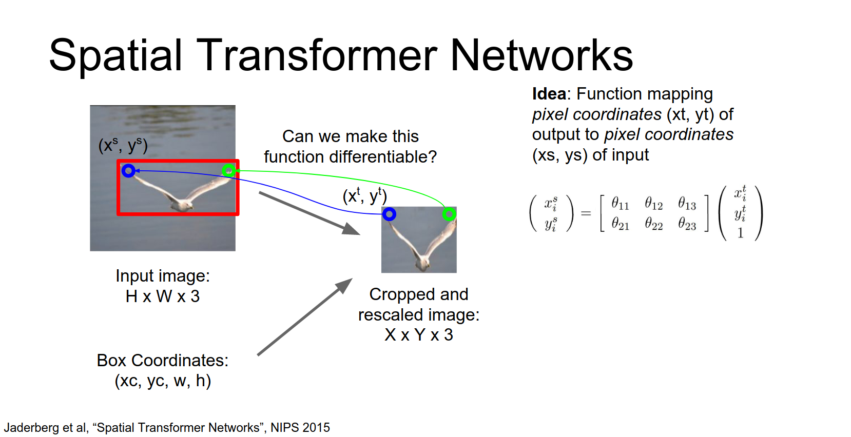
1. Grid Generator: Predict parameters \(\theta\) of an affine transform. Map output grid coordinates \((x^t, y^t)\) to input coordinates \((x^s, y^s)\).

We're going to write down a parameterized function that will map from coordinates of pixels in the output to coordinates of pixels in the input.

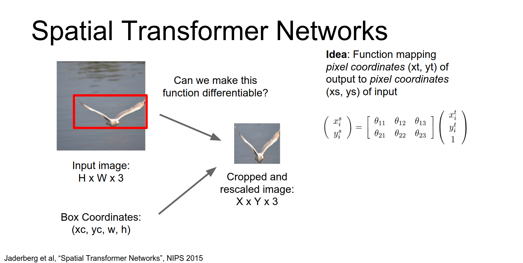
This upper right-hand pixel in the output image has the coordinates \(x^{t}\), \(y^{t}\) in the output.

And we're going to compute these coordinates \(x^{s}\) and \(y^{s}\) in the input image using this parameterized affine function.

So that's a nice differentiable function that we can differentiate with respect to these affine transform coordinates.

Then we can repeat this process and again for maybe the upper left hand pixel in the output image we again use this parameterized function to map to the coordinates of the pixel in the input.

1. Sampler: Use bilinear interpolation to sample pixel values from the input at the computed coordinates.

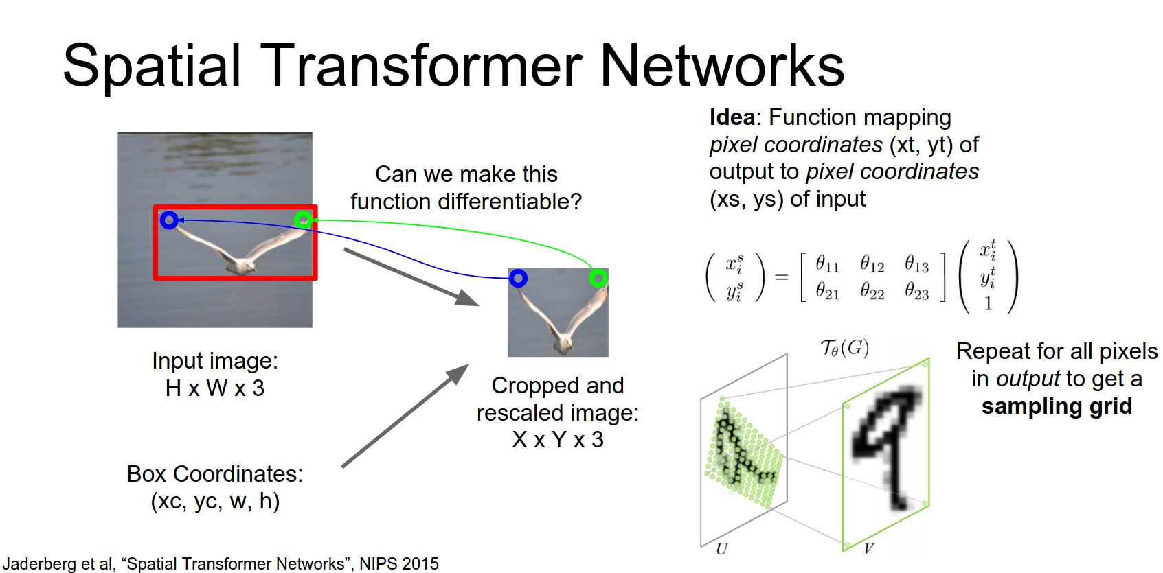
They take this idea from texture mapping in computer graphics and just use bilinear interpolation to compute the output once we have this sampling grid.

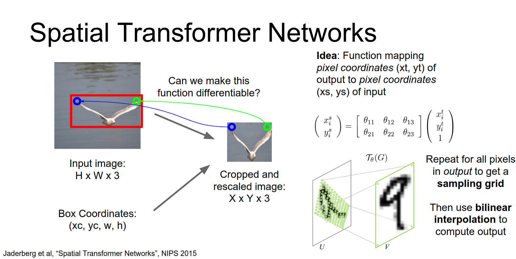
This entire process is differentiable!

The Spatial Transformer module:

• Localization Net: Predicts \(\theta\).
• Grid Generator: Creates sampling grid.
• Sampler: Produces output map.

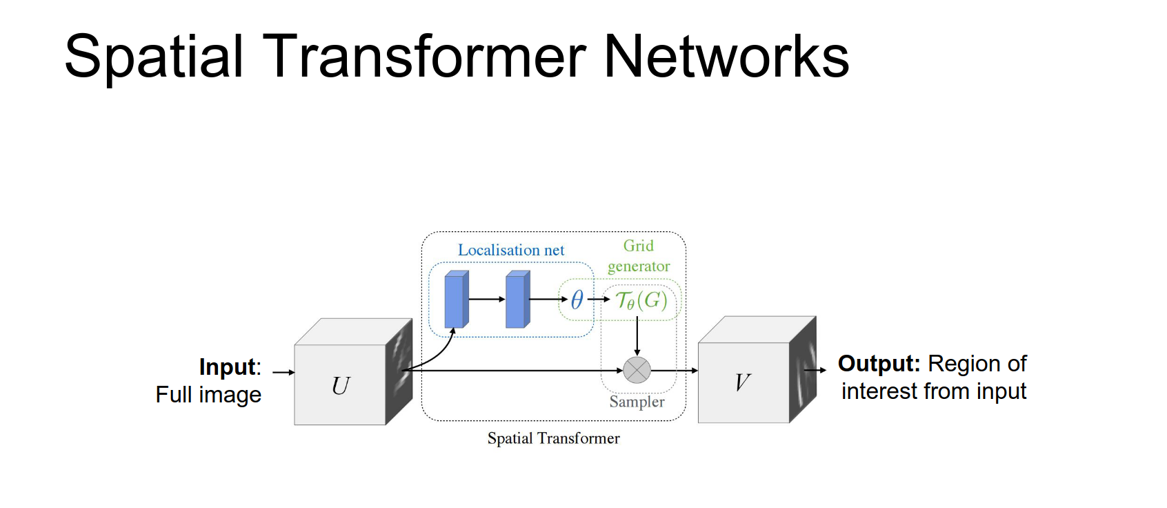
This localization network will actually produce as output these affine transform coordinates theta.

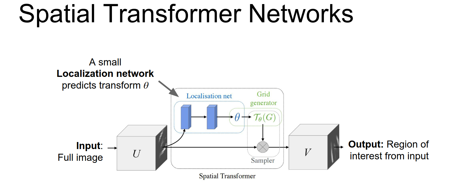
These affine transform coordinates will be used to compute a sampling grid.

So now that we've predicted these at this affine transform from the localization Network we map each pixel in the output the coordinates of each pixel in the output back to the input.

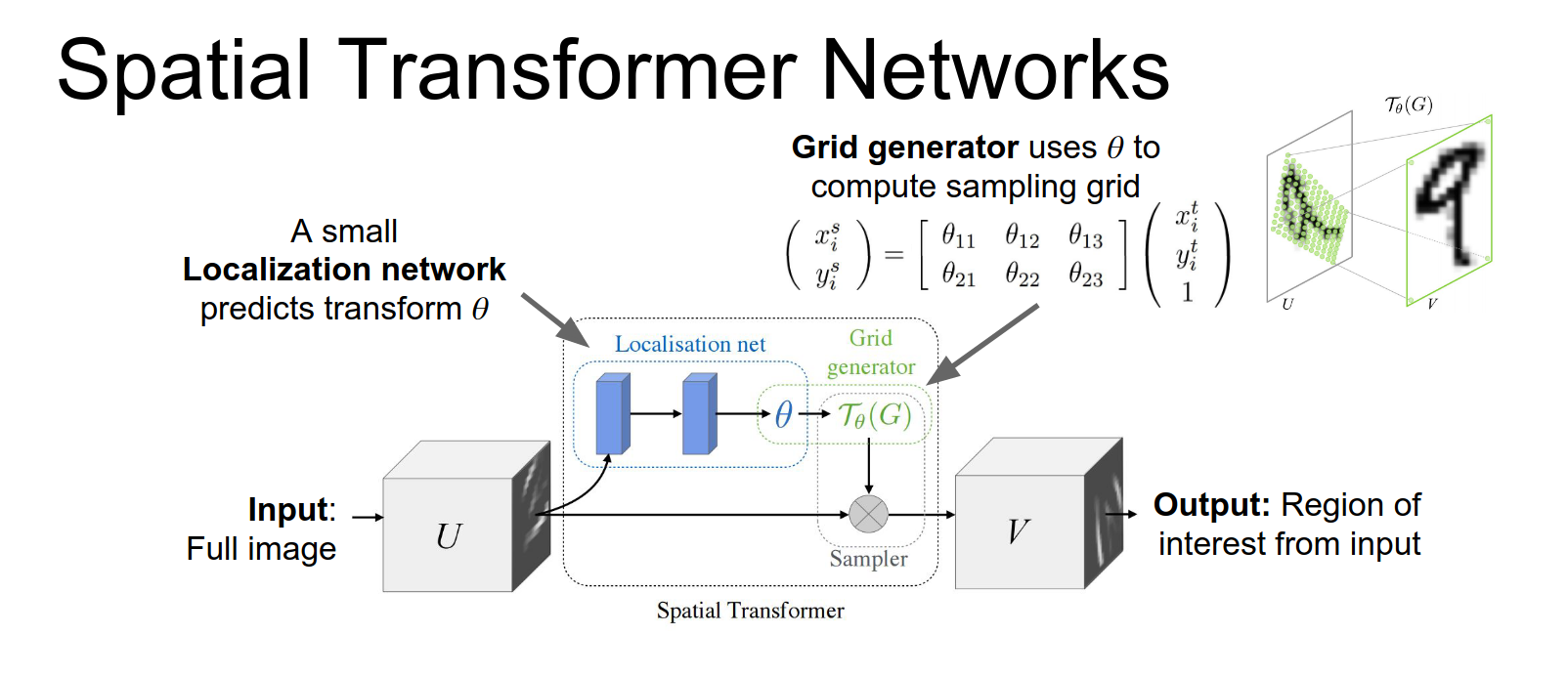
Now once we have the sampling grid, we can just apply bilinear interpolation to compute the values in the pixels of the output.

It's clear that every single part of this network is one continuous and two differentiable.

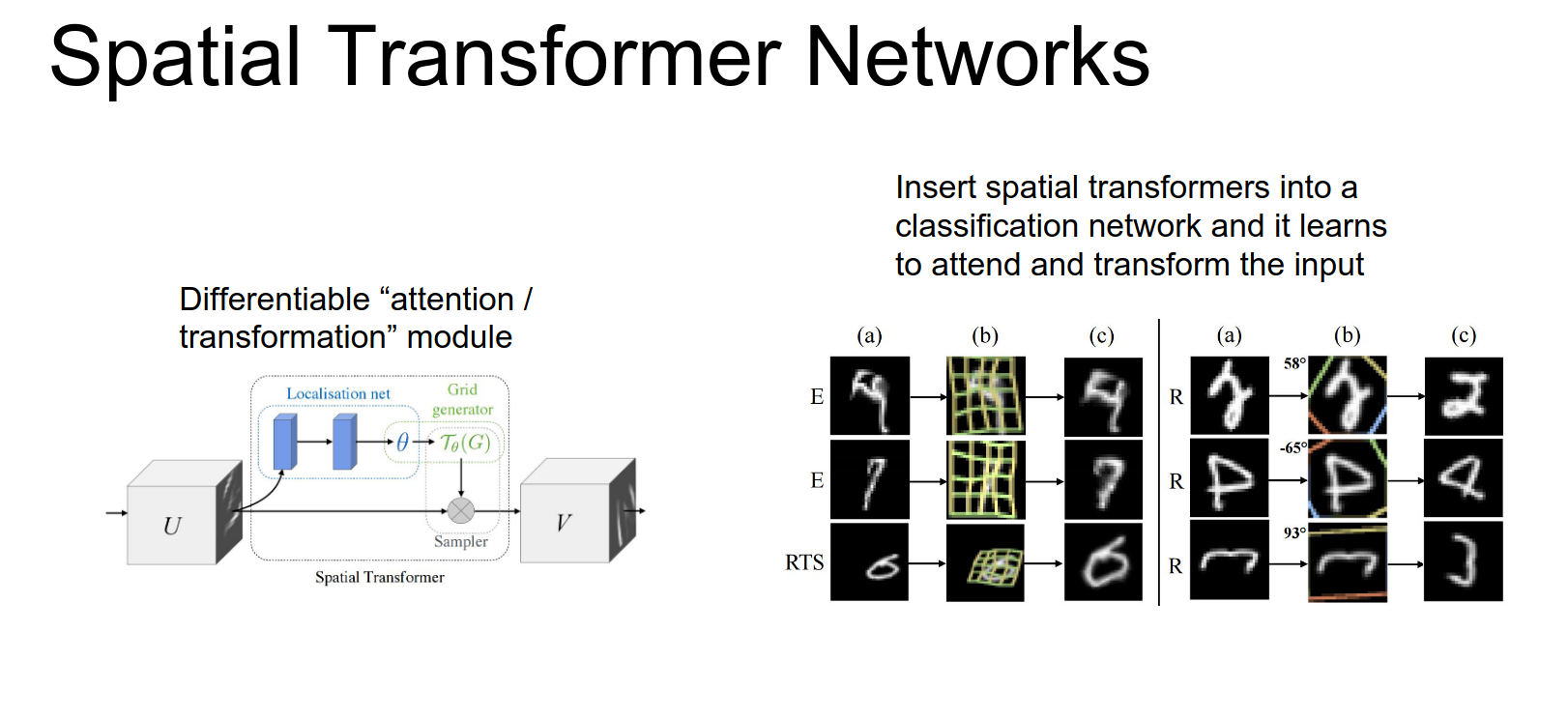
Once you have this spatial distance spatial transform or module we can just insert it into existing networks to sort of let them learn to attends to things.

They actually consider several other more complicated transforms not just these affine transforms you could also imagine that so that's the mapping from your output pixels back to your input pixels on the previous slide we showed an affine transform, but they also consider projective transforms and also thin plate splines.

But the idea is you just want some parameterize and differentiable function and you could go crazy with that part.

Here on the left the network is just trying to classify these digits that are warped. On the Left we have different versions of warped digits on this middle column is showing these different thin plate splines that it's using to attends to a part of the image, and then on the right it shows the output of the spatial transformer module.

Which has not only attended to that region but also unwarped it corresponding to examine those splines.

And on the right is using an affine transform not these thin plate splines. So you can see that this is actually doing more than just attending to the input we're actually transforming the input as well. So for example in this middle column this is a 4 but it's actually rotated by something by something like 90 degrees.

by using this affine transform the network can not only attends to the 4 but also rotate it into the proper position for the downstream classification Network.

And this is all very cool and again sort of similar to the soft attention, we don't need explicit supervision it can just decide for itself where it wants to attend in order to solve the problem.

Results:

• Classification: Learns to zoom in and un-rotate digits (canonicalization) without explicit supervision.
• Co-localization: Learns to find multiple objects.

So these guys have a video as well.

In the video you can see that, it's running a classification task but we're varying the input continuously.

When we rotate that digit and the network actually learns to unrotate digit and canonicalize the pose.

Both with affine transforms or thin placed blinds this is using even crazier warping with projective transforms so you can see that it does a really good job of learning to attend and also to unwarp.

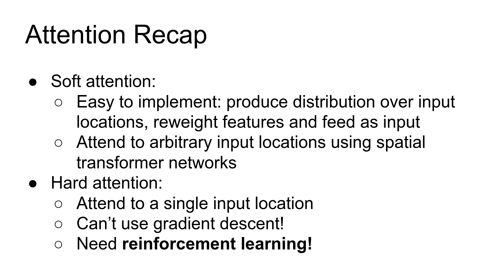
Summary of Attention:

• Soft Attention: Easy to implement, differentiable, constrained to grid.
• Hard Attention: Saves computation, requires Reinforcement Learning.
• Spatial Transformers: Differentiable way to attend to and transform arbitrary regions.

Done with lecture 13!